Chapter 2 Exact Dynamic Programming

In Chapter 1, we introduced the basic formulation of the finite-horizon and discrete-time optimal control problem, presented the Bellman principle of optimality, and derived the dynamic programming (DP) algorithm. We mentioned that, despite being a general-purpose algorithm, it can be difficult to implement DP exactly in practical applications.

In this Chapter, we will introduce two problem setups where DP can in fact be implemented exactly.

2.1 Linear Quadratic Regulator

Consider a linear discrete-time dynamical system $$\begin{equation} x_{k+1} = A_k x_k + B_k u_k + w_k, \quad k=0,1,\dots,N-1, \tag{2.1} \end{equation}$$ where $x_k \in \mathbb{R}^n$ the state, $u_k \in \mathbb{R}^m$ the control, $w_k \in \mathbb{R}^n$ the independent, zero-mean disturbance with given probability distribution that does not depend on $x_k,u_k$, and $A_k \in \mathbb{R}^{n \times n}, B_k \in \mathbb{R}^{n \times m}$ are known matrices determining the transition dynamics.

We want to solve the following optimal control problem $$\begin{equation} \min_{\mu_0,\dots,\mu_{N-1}} \mathbb{E} \left\{ x_N^T Q_N x_N + \sum_{k=0}^{N-1} \left( x_k^T Q_k x_k + u_k^T R_k u_k \right) \right\}, \tag{2.2} \end{equation}$$ where the expectation is taken over the randomness in $w_0,\dots,w_{N-1}$. In (2.2), $\{Q_k \}_{k=0}^N$ are positive semidefinite matrices, and $\{ R_k \}_{k=0}^{N-1}$ are positive definite matrices. The formulation (2.2) is typically known as the linear quadratic regulator (LQR) problem because the dynamics is linear, the cost is quadratic, and the formulation can be considered to “regulate” the system around the origin $x=0$.

We will now show that the DP algorithm in Theorem 1.2 can be exactly implemented for LQR.

The DP algorithm computes the optimal cost-to-go backwards in time. The terminal cost is $$J_N(x_N) = x_N^T Q_N x_N$$ by definition.

The optimal cost-to-go at time $N-1$ is equal to $$\begin{equation} \begin{split} J_{N-1}(x_{N-1}) = \min_{u_{N-1}} \mathbb{E}_{w_{N-1}} \{ x_{N-1}^T Q_{N-1} x_{N-1} + u_{N-1}^T R_{N-1} u_{N-1} + \\ \Vert \underbrace{A_{N-1} x_{N-1} + B_{N-1} u_{N-1} + w_{N-1} }_{x_N} \Vert^2_{Q_N} \} \end{split} \tag{2.3} \end{equation}$$ where $\Vert v \Vert_Q^2 = v^T Q v$ for $Q \succeq 0$. Now observe that the objective in (2.3) is $$\begin{equation} \begin{split} x_{N-1}^T Q_{N-1} x_{N-1} + u_{N-1}^T R_{N-1} u_{N-1} + \Vert A_{N-1} x_{N-1} + B_{N-1} u_{N-1} \Vert_{Q_N}^2 + \\ \mathbb{E}_{w_{N-1}} \left[ 2(A_{N-1} x_{N-1} + B_{N-1} u_{N-1} )^T Q_{N-1} w_{N-1} \right] + \\ \mathbb{E}_{w_{N-1}} \left[ w_{N-1}^T Q_N w_{N-1} \right] \end{split} \end{equation}$$ where the second line is zero due to $\mathbb{E}(w_{N-1}) = 0$ and the third line is a constant with respect to $u_{N-1}$. Consequently, the optimal control $u_{N-1}^\star$ can be computed by setting the derivative of the objective with respect to $u_{N-1}$ equal to zero $$\begin{equation} u_{N-1}^\star = - \left[ \left( R_{N-1} + B_{N-1}^T Q_N B_{N-1} \right)^{-1} B_{N-1}^T Q_N A_{N-1} \right] x_{N-1}. \tag{2.4} \end{equation}$$ Plugging the optimal controller $u^\star_{N-1}$ back to the objective of (2.3) leads to $$\begin{equation} J_{N-1}(x_{N-1}) = x_{N-1}^T S_{N-1} x_{N-1} + \mathbb{E} \left[ w_{N-1}^T Q_N w_{N-1} \right], \tag{2.5} \end{equation}$$ with $$S_{N-1} = Q_{N-1} + A_{N-1}^T \left[ Q_N - Q_N B_{N-1} \left( R_{N-1} + B_{N-1}^T Q_N B_{N-1} \right)^{-1} B_{N-1}^T Q_N \right] A_{N-1}.$$ We note that $S_{N-1}$ is positive semidefinite (this is an exercise for you to convince yourself).

Now we realize that something surprising and nice has happened.

1. The optimal controller $u^{\star}_{N-1}$ in (2.4) is a linear feedback policy of the state $x_{N-1}$, and

2. The optimal cost-to-go $J_{N-1}(x_{N-1})$ in (2.5) is quadratic in $x_{N-1}$, just the same as $J_{N}(x_N)$.

This implies that, if we continue to compute the optimal cost-to-go at time $N-2$, we will again compute a linear optimal controller and a quadratic optimal cost-to-go. This is the rare nice property for the LQR problem, that is,

The (representation) complexity of the optimal controller and cost-to-go does not grow as we run the DP recursion backwards in time.

We summarize the solution for the LQR problem (2.2) as follows.

Proposition 2.1 (Solution of Discrete-Time Finite-Horizon LQR) The optimal controller for the LQR problem (2.2) is a linear state-feedback policy $$\begin{equation} \mu_k^\star(x_k) = - K_k x_k, \quad k=0,\dots,N-1. \tag{2.6} \end{equation}$$ The gain matrix $K_k$ can be computed as $$K_k = \left( R_k + B_k^T S_{k+1} B_k \right)^{-1} B_k^T S_{k+1} A_k,$$ where the matrix $S_k$ satisfies the following backwards recursion $$\begin{equation} \hspace{-6mm} \begin{split} S_N &= Q_N \\ S_k &= Q_k + A_k^T \left[ S_{k+1} - S_{k+1}B_k \left( R_k + B_k^T S_{k+1} B_k \right)^{-1} B_k^T S_{k+1} \right] A_k, k=N-1,\dots,0. \end{split} \tag{2.7} \end{equation}$$ The optimal cost-to-go is given by $$J_0(x_0) = x_0^T S_0 x_0 + \sum_{k=0}^{N-1} \mathbb{E} \left[ w_k^T S_{k+1} w_k\right].$$ The recursion (2.7) is called the discrete-time Riccati equation.

Proposition 2.1 states that, to evaluate the optimal policy (2.6), one can first run the backwards Riccati equation (2.7) to compute all the positive definite matrices $S_k$, and then compute the gain matrices $K_k$. For systems of reasonable dimensions, evalutating the matrix inversion in (2.7) should be fairly efficient.

2.1.1 Infinite-Horizon LQR

In many robotics applications, it is often more useful to study the infinite-horizon LQR problem $$\begin{align} \min_{u_k} & \quad \sum_{k=0}^{\infty} \left( x_k^T Q x_k + u_k^T R u_k \right) \tag{2.8} \\ \text{subject to} & \quad x_{k+1} = A x_k + B u_k, \quad k=0,\dots,\infty, \tag{2.9} \end{align}$$ where $Q \succeq 0$, $R \succ 0$, and $A,B$ are constant matrices. The reason for studying the formulation (2.8) is twofold. First, for nonlinear systems, we often linearize the nonlinear dynamics around an (equilibrium) point we care about, leading to constant $A$ and $B$ matrices. Second, we care more about the asymptotic effect of our controller than its behavior in a fixed number of steps. We will soon see an example of this formulation for balancing a simple pendulum.

The infinite-horizon formulation is essentially the finite-horizon formulation (2.2) with $N \rightarrow \infty$. Based on our intuition in deriving the finite-horizon LQR solution, we may want to hypothesize that the optimal cost-to-go is a quadratic function $$\begin{equation} J_{k}(x_{k}) = x_{k}^T S x_{k}, k=0,\dots,\infty \tag{2.10} \end{equation}$$ for some positive definite matrix $S$, and proceed to invoke the DP algorithm. Notice that we hypothesize the matrix $S$ is in fact stationary, i.e., it does not change with respect to time. This hypothesis makes sense because the $A,B,Q,R$ matrices are stationary in the formulation (2.8). Invoking the DP algorithm we have $$\begin{equation} x_k^T S x_k = J_k(x_k) = \min_{u_k} \left\{ x_k^T Q x_k + u_k^T R u_k + \Vert \underbrace{A x_k + B u_k}_{x_{k+1}} \Vert_S^2 \right\}. \tag{2.11} \end{equation}$$ The minimization over $u_k$ in (2.11) can again be solved in closed-form by setting the gradient of the objective with respect to $u_k$ to be zero $$\begin{equation} u_k^\star = - \underbrace{\left[ \left( R + B^T S B \right)^{-1} B^T S A \right]}_{K} x_k. \tag{2.12} \end{equation}$$ Plugging the optimal $u_k^\star$ back into (2.11), we see that the matrix $S$ has to satisfy the following equation $$\begin{equation} S = Q + A^T \left[ S - SB \left( R + B^T S B \right)^{-1} B^T S \right] A. \tag{2.13} \end{equation}$$ Equation (2.13) is the famous algebraic Riccati equation.

Let’s zoom out to see what we have done. We started with a hypothetical optimal cost-to-go (2.10) that is stationary, and invoked the DP algorithm in (2.11), which led us to the algebraic Riccati equation (2.13). Therefore, if there actually exists a solution to the algebraic Riccati equation (2.13), then the linear controller (2.12) is indeed optimal (by the optimality of DP)!

So the question boils down to if the algebraic Riccati equation has a solution $S$ that is positive definite? The following proposition gives an answer.

Proposition 2.2 (Solution of Discrete-Time Infinite-Horizon LQR) Consider a linear system $$x_{k+1} = A x_k + B u_k,$$ with $(A,B)$ controllable (see Appendix C.2). Let $Q \succeq 0$ in (2.8) be such that $Q$ can be written as $Q = C^T C$ with $(A,C)$ observable.

Then the optimal controller for the infinite-horizon LQR problem (2.8) is a stationary linear policy $$\mu^\star (x) = - K x,$$ with $$K = \left( R + B^T S B \right)^{-1} B^T S A.$$ The matrix $S$ is the unique positive definite matrix that satisfies the algebraic Riccati equation $$S = Q + A^T \left[ S - SB \left( R + B^T S B \right)^{-1} B^T S \right] A.$$

Moreover, the closed-loop system $$x_{k+1} = A x_k + B (-K x_k) = (A - BK) x_k$$ is stable, i.e., the eigenvalues of the matrix $A - BK$ are strictly within the unit circle (see Appendix C.1.2).

A rigorous proof of Proposition 2.2 is available in Proposition 3.1.1 of (Bertsekas 2012). The proof basically studies the limit of the discrete-time Riccati equation (2.7) when $N \rightarrow \infty$. Indeed, the algebraic Riccati equation (2.13) is the limit of the discrete-time Riccati equation (2.7) when $N \rightarrow \infty$. The assumptions of $(A,B)$ being controllable and $(A,C)$ being observable can be relaxted to $(A,B)$ being stabilizable and $(A,C)$ being detectable (for definitions of stabilizability and detectability, see Appendix C).

We have not discussed how to solve the algebraic Riccati equation (2.7). It is clear that (2.7) is not a linear system of equations in $S$. In fact, the numerical algorithms for solving the algebraic Riccati equation can be highly nontrivial, for example see (Arnold and Laub 1984). Fortunately, such algorithms are often readily available, and as practitioners we do not need to worry about solving the algebraic Riccati equation by ourselves. For example, the Matlab dlqr function computes the $K$ and $S$ matrices from $A,B,Q,R$.

Let us now apply the infinite-horizon LQR solution to stabilizing a simple pendulum.

Example 2.1 (Pendulum Stabilization by LQR) Consider the simple pendulum in Fig. 2.1 with dynamics $$\begin{equation} x = \begin{bmatrix} \theta \\ \dot{\theta} \end{bmatrix}, \quad \dot{x} = f(x,u) = \begin{bmatrix} \dot{\theta} \\ -\frac{1}{ml^2}(b \dot{\theta} + mgl \sin \theta) + \frac{1}{ml^2} u \end{bmatrix} \tag{2.14} \end{equation}$$ where $m$ is the mass of the pendulum, $l$ is the length of the pole, $g$ is the gravitational constant, $b$ is the damping ratio, and $u$ is the torque applied to the pendulum.

We are interested in applying the LQR controller to balance the pendulum in the upright position $x_d = [\pi,0]^T$ with a zero velocity.

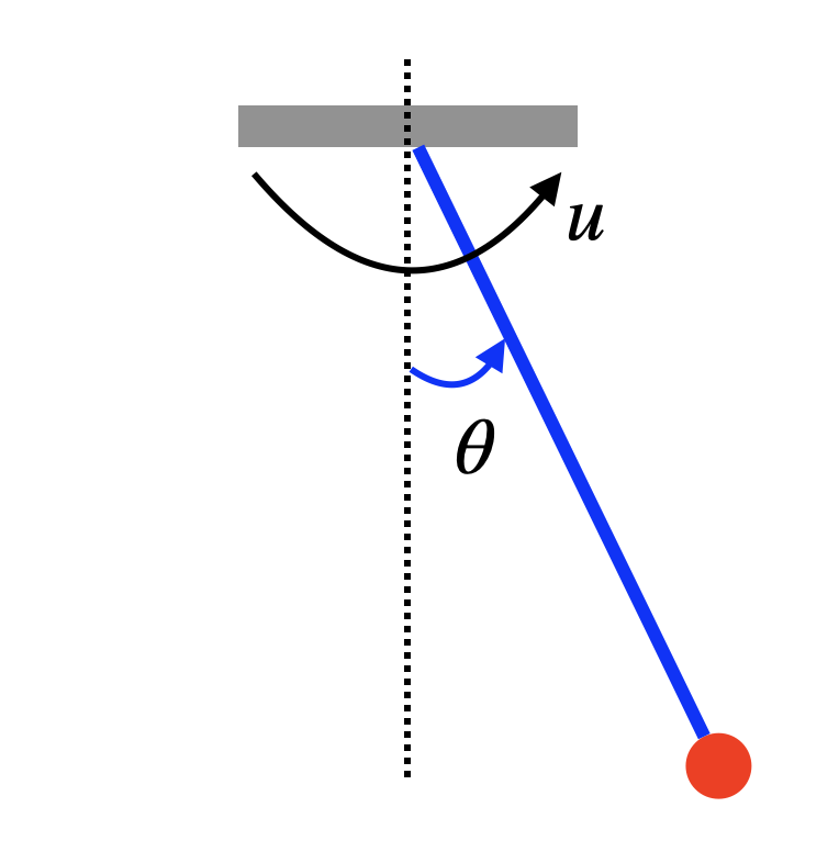
Figure 2.1: A Simple Pendulum.

Let us first shift the dynamics so that “$0$” is the upright position. This can be done by defining a new variable $z = x - x_d = [\theta - \pi, \dot{\theta}]^T$, which leads to $$\begin{equation} \dot{z} = \dot{x} = f(x,u) = f(z + x_d,u) = \begin{bmatrix} z_2 \\ \frac{1}{ml^2} \left( u - b z_2 + mgl \sin z_1 \right) \end{bmatrix} = f'(z,u). \tag{2.15} \end{equation}$$ We then linearize the nonlinear dynamics $\dot{z} = f'(z,u)$ at the point $z^\star = 0, u^\star = 0$: $$\begin{align} \dot{z} & \approx f'(z^\star,u^\star) + \left( \frac{\partial f'}{\partial z} \right)_{z^\star,u^\star} (z - z^\star) + \left( \frac{\partial f'}{\partial u} \right)_{z^\star,u^\star} (u - u^\star) \\ & = \begin{bmatrix} 0 & 1 \\ \frac{g}{l} \cos z_1 & - \frac{b}{ml^2} \end{bmatrix}_{z^\star, u^\star} z + \begin{bmatrix} 0 \\ \frac{1}{ml^2} \end{bmatrix} u \\ & = \underbrace{\begin{bmatrix} 0 & 1 \\ \frac{g}{l} & - \frac{b}{ml^2} \end{bmatrix}}_{A_c} z + \underbrace{\begin{bmatrix} 0 \\ \frac{1}{ml^2} \end{bmatrix}}_{B_c} u. \end{align}$$ Finally, we convert the continuous-time dynamics to discrete time with a fixed discretization $h$ $$z_{k+1} = \dot{z}_k \cdot h + z_k = \underbrace{(h \cdot A_c + I )}_{A} z_k + \underbrace{(h \cdot B_c)}_{B} u_k.$$

We are now ready to implement the LQR controller. In the formulation (2.8), we choose $Q = I$, $R = I$, and solve the gain matrix $K$ using the Matlab dlqr function.

Fig. 2.2 shows the simulation result for $m=1,l=1,b=0.1$, $g = 9.8$, and $h = 0.01$, with an initial condition $z^0 = [0.1,0.1]^T$. We can see that the LQR controller successfully stabilizes the pendulum at $z^\star$, the upright position.

You can play with the Matlab code here.

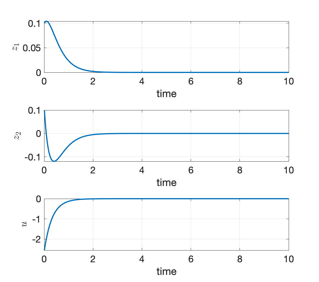
Figure 2.2: LQR stabilization of a simple pendulum.

2.1.2 LQR with Constraints

Let’s explore LQR with constraints in Exercise 9.2

2.2 Markov Decision Process

In Section 2.1, we see that linear dynamics and quadratic costs leads to exact dynamic programming. We now introduce another setup where the number of states and controls is finite (as opposed to the LQR case where $x_k$ and $u_k$ live in continuous spaces). We will see that we can execute DP exactly in this setup as well.

Optimal control in the case of finite states and controls is typically introduced in the framework of a Markov Decision Process (MDP, which is common in Reinforcement Learning). There are many variations of a MDP, and here we only focus on the discounted infinite-horizon MDP. For a more complete treatment of MDPs, I suggest checking out this course at Harvard.

Formally, a discounted infinite-horizon MDP $\mathcal{M} = (\mathbb{X},\mathbb{U},P,g,\gamma,\sigma)$ is specified by

• a state space $\mathbb{X}$ that is finite with size $|\mathbb{X}|$

• a control space $\mathbb{U}$ that is finite with size $|\mathbb{U}|$

• a transition function $P: \mathbb{X} \times \mathbb{U} \rightarrow \Delta(\mathbb{X})$, where $\Delta(\mathbb{X})$ is the space of probability distributions over $\mathbb{X}$; specifically, $P(x' \mid x, u)$ is the probability of transitioning into state $x'$ from state $x$ using control $u$. If the system is deterministic, then $P(x' \mid x, u)$ is nonzero only for a single next state $x'$

• a cost function $g: \mathbb{X} \times \mathbb{U} \rightarrow [0,1]$; $g(x,u)$ is the cost of taking the control $u$ at state $x$

• a discount factor $\gamma \in [0,1)$

• an initial state distribution $\sigma \in \Delta(\mathbb{X})$ that specifies how the initial state $x_0$ is generated; in many cases we will assume $x_0$ is fixed and $\sigma$ is a distribution supported only on $x_0$.

In an MDP, the system starts at some state $x_0 \sim \sigma$. At each step $k = 0,1,2,\dots$, the system decides a control $u_k \in \mathbb{U}$ and incurs a cost $g(s_k,u_k)$. The control $u_k$ brings the system into a new state $x_{k+1} \sim P(\cdot \mid x_k, u_k)$, at which the controller decides a new control $u_{k+1}$. This process continues forever.

Controller (policy). In general, a time-varying controller $\pi = (\pi_0,\dots,\pi_k,\dots)$ is a mapping from all previous states and controls to a distribution over current controls. The mapping $\pi_k$ at timestep $k$ is $$\pi_k: (x_0,u_0,x_1,u_1,\dots,x_k) \mapsto u_k \sim q_k \in \Delta(\mathbb{U}).$$ Note that $u_k$ can be randomized and it is drawn from a distribution $q_k$ supported on the set of controls $\mathbb{U}$. A stationary controller (policy) $\pi: \mathbb{X} \rightarrow \Delta(\mathbb{U})$ specifies a decison-making strategy that is purely based on the current state $x_k$. A deterministic and stationary controller $\pi: \mathbb{X} \rightarrow \mathbb{U}$ excutes a deterministic control $u_k$ at each step.

Cost-to-go and $Q$-value. Given a controller $\pi$ and an initial state $x_0$, we associate with it the following discounted infinite-horizon cost $$\begin{equation} J_\pi(x_0) = \mathbb{E} \left\{ \sum_{k=0}^{\infty} \gamma^k g(x_k, u_k^{\pi}) \right\}, \tag{2.16} \end{equation}$$ where the expectation is taken over the randomness of the transition $P$ and the controller $\pi$. Note that we have used $u^{\pi}_k$ to denote the control at step $k$ by following the controller $\pi$. Similarly, we define the $Q$-value function as $$\begin{equation} Q_\pi(x_0,u_0) = \mathbb{E} \left\{ g(x_0,u_0) + \sum_{k=1}^{\infty} \gamma^k g(x_k,u_k^{\pi}) \right\}. \tag{2.17} \end{equation}$$ The difference between $Q_\pi(x_0,u_0)$ and $J_\pi(x_0)$ is that at step zero, $J_\pi(x_0)$ follows the controller $\pi$ while $Q_\pi(x_0,u_0)$ assumes the control $u_0$ is given. By the assumption that $g(x_k,u_k) \in [0,1]$, we have $$0 \leq J_\pi(x_0), Q_\pi(x_0,u_0) \leq \sum_{k=0}^{\infty} \gamma^k = \frac{1}{1-\gamma}, \quad \forall \pi.$$

Our goal is to find the best controller that minimizes the cost function $$\begin{equation} \pi^\star \in \arg\min_{\pi \in \Pi} J_\pi(x_0) \tag{2.18} \end{equation}$$ for a given initial state $x_0$, where $\Pi$ is the space of all non-stationary and randomized controllers.

A remarkable property of MDPs is that there exists an optimal controller that is stationary and deterministic.

Theorem 2.1 (Deterministic and Stationary Optimal Policy) Let $\Pi$ be the space of all non-stationary and randomized policies. Define $$J^\star_\pi(x) = \min_{\pi \in \Pi} J_\pi(x), \quad Q^\star_\pi(x,u) = \min_{\pi \in \Pi } Q_\pi(x,u).$$ There exists a deterministic and stationary policy $\pi^\star$ such that for all $x \in \mathbb{X}$ and $u \in \mathbb{U}$, $$J_{\pi^\star}(x) = J^\star(x), \quad Q_{\pi^\star}(x,u) = Q^\star(x,u).$$ We call such a policy $\pi$ an optimal policy.

Proof. See Theorem 1.7 in (Agarwal et al. 2022).

This Theorem shows that we can restrict ourselves to stationary and deterministic policies without losing performance.

In the next, we show how to characterize the optimal policy and value function.

2.2.1 Bellman Optimality Equations

We now restrict ourselves to stationary policies. We first introduce the Bellman Consistency Equations for stationary policies.

Lemma 2.1 (Bellman Consistency Equations) Let $\pi$ be a stationary policy. Then $J_\pi$ and $Q_\pi$ satisfy the following Bellman consistency equations $$\begin{align} J_\pi(x) &= \mathbb{E}_{u \sim \pi(\cdot \mid x)} Q_\pi(x,u), \tag{2.19} \\ Q_\pi(x,u) &=g(x,u) + \gamma \mathbb{E}_{x' \sim P(\cdot \mid x,u)} J_\pi(x'). \tag{2.20} \end{align}$$

Proof. By the definition of the cost-to-go function in (2.16), we have $$J_\pi(x_0) = \mathbb{E}\left\{ \sum_{k=0}^{\infty} \gamma^k g(x_k, \pi(x_k)) \right\} = \mathbb{E}_{u_0 \sim \pi(\cdot \mid x_0)} \underbrace{\mathbb{E} \left\{ g(x_0,u_0) + \sum_{k=1}^{\infty} \gamma^k g(x_k,\pi(x_k)) \right\}}_{Q_\pi(x_0,u_0)}.$$ The above equation holds for any $x_0$, proving (2.19).

To show (2.20), we recall the definition of the $Q$-value function (2.17) $$\begin{align} Q_\pi(x_0,u_0) & = \mathbb{E} \left\{ g(x_0,u_0) + \sum_{k=1}^{\infty} \gamma^k g(x_k,\pi(x_k)) \right\} \\ &= g(x_0,u_0) + \gamma \mathbb{E} \left\{ \sum_{k=1}^{\infty} \gamma^{k-1} g(x_k,\pi(x_k)) \right\} \tag{2.21} \end{align}$$ Now observe that the expectation of the second term in (2.21) is taken over both the randomness of $x_1$ and the randomness of the policy after $x_1$ is reached. Therefore, $$\mathbb{E} \left\{ \sum_{k=1}^{\infty} \gamma^{k-1} g(x_k,\pi(x_k)) \right\} = \mathbb{E}_{x_1 \sim P(\cdot \mid x_0,u_0)} \underbrace{\left\{ \mathbb{E} \left\{ \sum_{k=1}^{\infty} \gamma^{k-1} g(x_1,\pi(x_1)) \right\} \right\}}_{J_\pi(x_1)}.$$ Plugging the above equation back to (2.21), we obtain the desired result in (2.20).

Matrix Representation. It is useful to think of $P,g,J_\pi,Q_\pi$ as matrices. In particular, the transition function $P$ can be considered as a matrix of dimension $|\mathbb{X}||\mathbb{U}| \times \mathbb{X}$, where $$P_{(x,u),x'} = P(x' \mid x,u)$$ is the entry of $P$ at the row $(x,u)$ (there are $|\mathbb{X}||\mathbb{U}|$ such rows) and column $x'$ (there are $|\mathbb{X}|$ such columns). The running cost $g$ is vector of $|\mathbb{X}||\mathbb{U}|$ entries. The cost-to-go $J_\pi(x)$ is a vector of $|\mathbb{X}|$ entries. The $Q$-value function $Q_\pi(x,u)$ is a vector of $|\mathbb{X}||\mathbb{U}|$ entries. We also introduce $P^{\pi}$ with dimension $|\mathbb{X}||\mathbb{U}| \times |\mathbb{X}||\mathbb{U}|$ as the transition matrix induced by a stationary policy $\pi$. In particular, $$P^\pi_{(x,u),(x',u')} = P(x' \mid x,u) \pi(u'\mid x').$$ In words, $P^\pi_{(x,u),(x',u')}$ is the probability that $(x',u')$ follows $(x,u)$.

With the matrix representation, we can compactly write the Bellman consistency equation (2.20) as $$\begin{equation} Q_\pi = g + \gamma P J_\pi. \tag{2.22} \end{equation}$$ We can also combine (2.19) and (2.20) together and write $$Q_\pi(x,u) = g(x,u) + \gamma \mathbb{E}_{x' \sim P(\cdot \mid x,u)} \left\{ \mathbb{E}_{u' \sim \pi(\cdot \mid x')} Q_\pi(x',u') \right\} = g(x,u) + \gamma \mathbb{E}_{(x',u') \sim P^\pi(\cdot \mid (x,u))} Q_\pi(x',u'),$$ which, using matrix representation, becomes $$\begin{equation} Q_\pi = g + \gamma P^\pi Q_\pi. \tag{2.23} \end{equation}$$ Equation (2.23) immediately yields $$\begin{equation} Q_\pi = (I - \gamma P^\pi)^{-1} g, \tag{2.24} \end{equation}$$ that is, the $Q$-value function associated with a stationary policy $\pi$ can be simply computed from solving a linear system as in (2.24).³

Lemma 2.1, together with the equivalent matrix equations (2.22) and (2.23), provide the conditions that $J_\pi$ and $Q_\pi$, induced by any stationary policy $\pi$, need to satisfy. In the next, we describe the conditions that characterize the optimal policy.

Theorem 2.2 (Bellman Optimality Equations) A vector $Q \in \mathbb{R}^{|\mathbb{X}||\mathbb{U}|}$ is said to satisfy the Bellman optimality equation if $$\begin{equation} Q(x,u) = g(x,u) + \gamma \mathbb{E}_{x' \sim P(\cdot \mid x,u)} \left\{ \min_{u' \in \mathbb{U}} Q(x',u') \right\}, \quad \forall (x,u) \in \mathbb{X} \times \mathbb{U}. \tag{2.25} \end{equation}$$

A vector $Q^\star$ is the optimal $Q$-value function if and only if it satisfies (2.25). Moreover, the deterministic policy defined by $$\pi^\star(x) \in \arg\min_{u \in \mathbb{U}} Q^\star(x,u)$$ with ties broken arbitrarily is an optimal policy.

Proof. See Theorem 1.8 in (Agarwal et al. 2022).

We now make a few definitions to interpret Theorem 2.2. For any vector $Q \in \mathbb{R}^{|\mathbb{X}||\mathbb{U}|}$, define the greedy policy as $$\begin{equation} \pi_{Q}(x) \in \arg\min_{u \in \mathbb{U}} Q(x,u) \tag{2.26} \end{equation}$$ with ties broken arbitrarily. With this notation, by Theorem 2.2, the optimal policy is $$\pi^\star = \pi_{Q^\star},$$ where $Q^\star$ is the optimal $Q$-value function. Similarly, let us define $$J_Q(x) = \min_{u \in \mathbb{U}} Q(x,u).$$ Note that $J_Q$ has dimension $|\mathbb{X}|$. With these notations, the Bellman optimality operator is defined as $$\begin{equation} \mathcal{T}Q = g + \gamma P J_Q, \tag{2.27} \end{equation}$$ which is nothing but a matrix representation of the right-hand side of (2.25). This allows us to concisely write the Bellman optimality equation (2.25) as $$\begin{equation} Q = \mathcal{T}Q. \tag{2.28} \end{equation}$$ Therefore, an equivalent way to interpret Theorem 2.2 is that $Q = Q^\star$ if and only if $Q$ is a fixed point to the Bellman optimality operator $\mathcal{T}$.

2.2.2 Value Iteration

Intepreting the optimal $Q$-value function as the fixed point to the Bellman optimality operator (2.28) leads us to a natural algorithm for solving the optimal control problem.

We start with $Q^{(0)}$ being an all-zero vector and then at iteration $t$, we perform $$Q^{(t+1)} \leftarrow \mathcal{T} Q^{(t)},$$ with $\mathcal{T}$ defined in (2.27). Let us observe the simplicity of this algorithm: at each iteration, one only needs to perform $\min_{u \in \mathbb{U}} Q^{(t)}(x,u)$, which is very efficient when $|\mathbb{U}|$ is not too large.

The next theorem states this simple algorithm converges to the optimal value function.

Theorem 2.3 (Value Iteration) Set $Q^{(0)} = 0$. For $t=0,\dots$, perform $$Q^{(t+1)} \leftarrow \mathcal{T} Q^{(t)}.$$ Let $\pi^{(k)} = \pi_{Q^{(k)}}$ (see the definition in (2.26)). For $t \geq \frac{\log \frac{2}{(1-\gamma)^2 \epsilon}}{1-\gamma}$, we have $$J^{\pi^{(t)}} \leq J^\star + \epsilon \mathbb{1},$$ where $\mathbb{1}$ is the all-ones vector.

Essentially, the value function obtained from value iteration converges to the optimal cost-to-go.

Let us use an example to appreciate this algorithm.

Example 2.2 (Shortest Path in Grid World) Consider the following $10 \times 10$ grid world, where the top-right cell is the goal location, and the dark blue colored cells are obstacles.

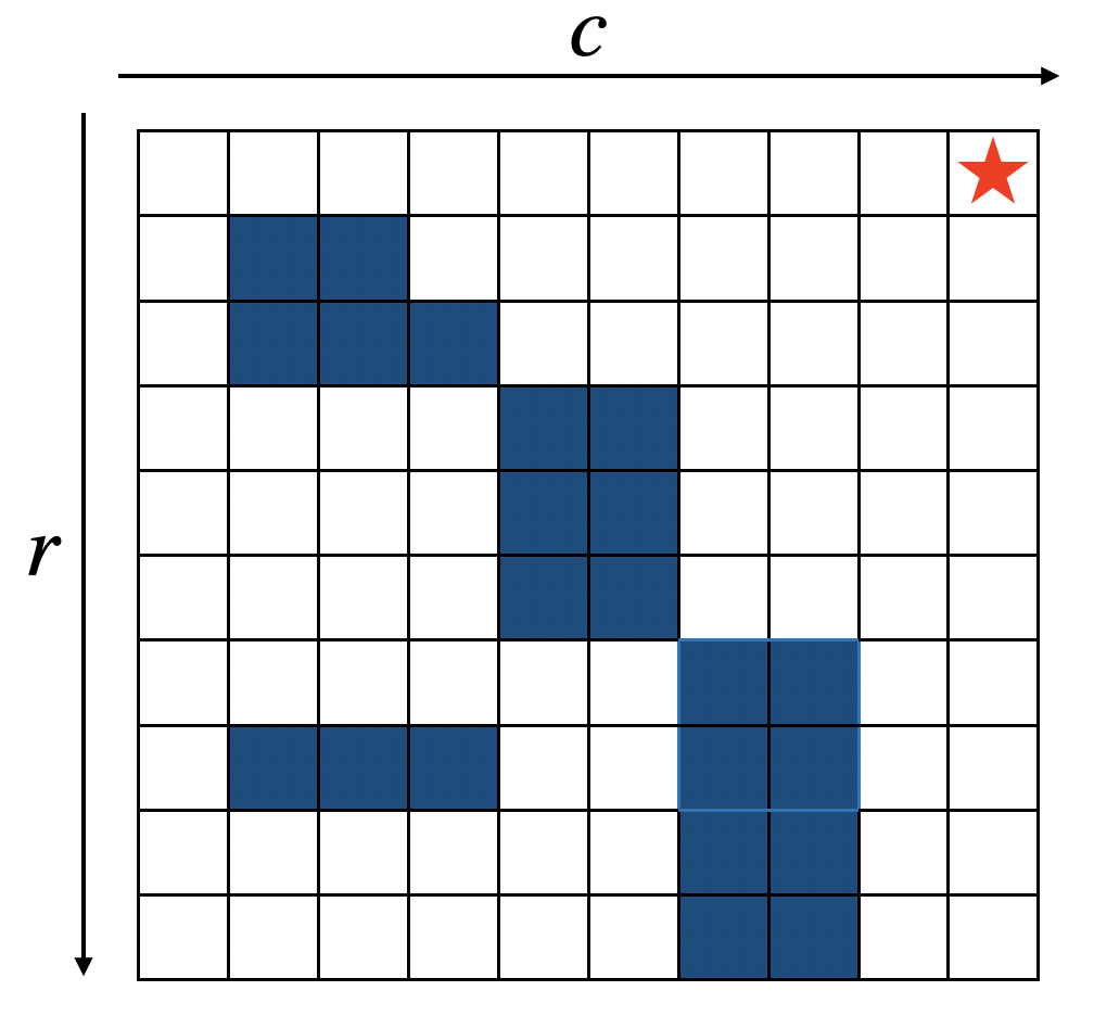
Figure 2.3: Grid World with Obstacles.

We want to find the shortest path from a given cell to the target cell, while not hitting obstacles.

To do so, we set the state space of the system as $$\mathbb{X} = \left\{ \begin{bmatrix} r \\ c \end{bmatrix} \middle\vert r,c \in \{ 1,\dots,10 \} \right\}$$ where $r$ is the row index (from top to bottom) and $c$ is the column index (from left to right). The control space is moving left, right, up, down, or do nothing: $$\mathbb{U} = \left\{ \begin{bmatrix} 1 \\ 0 \end{bmatrix}, \begin{bmatrix} -1 \\ 0 \end{bmatrix}, \begin{bmatrix} 0 \\ 1 \end{bmatrix}, \begin{bmatrix} 0 \\ -1 \end{bmatrix}, \begin{bmatrix} 0 \\ 0 \end{bmatrix} \right\}.$$ The system dynamics is deterministic $$x' = \begin{cases} x + u & \text{if } x + u \text{ is inside the grid} \\ x & \text{otherwise} \end{cases}.$$ We then design the following running cost function $g$ $$g(x,u) = \begin{cases} 0 & \text{if } x = [1,10]^T \text{ is the target} \\ 20 & \text{if } x \text{ is an obstacle} \\ 1 & \text{otherwise} \end{cases}.$$ Note that $g(x,u)$ defined above does not even satisfy $g \in [0,1]$. We then use value iteration to solve the optimal control problem with $\gamma = 1$ $$J(x_0) = \min_{\pi} \sum_{k=0}^{\infty} g(x_k,\pi(x_k)).$$

The Matlab script of value iteration converges in $27$ iterations, and we obtain the optimal cost-to-go in Fig. 2.4.

Starting from the cell $[8,5]^T$, the red line in Fig. 2.4 plots the optimal trajectory that clearly avoids the obstacles.

Feel free to play with the size of the grid and the number of obstacles.

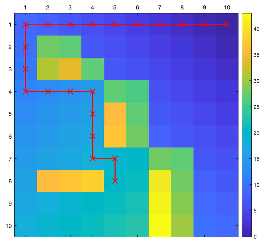
Figure 2.4: Optimal cost-to-go and an optimal trajectory.

Example 2.2 shows the simplicity and power of value iteration. However, the states and controls in the grid world are naturally discrete and finite. Is it possible to apply value iteration to optimal control problems where the states and controls live in continuous spaces?

2.2.3 Value Iteration with Barycentric Interpolation

Let us consider the discrete-time dynamics $$x_{k+1} = f(x_k, u_k)$$ where both $x_k$ and $u_k$ live in a continuous space, say $\mathbb{R}^{n}$ and $\mathbb{R}^m$, respectively.

A natural idea to apply value iteration is to discretize the state space and control space. For example, suppose $x \in \mathbb{R}^2$ and we have discretized $\mathbb{R}^2$ using $N$ points $$\mathcal{S} = \{s_1,\dots,s_N\}$$ that lie on a 2D grid, as shown in Fig. 2.5. Assume $x_k \in \mathcal{S}$ lies on the mesh grid, the next state $x_{k+1} = f(x_k,u_k)$ will, however, most likely not lie exactly on one of the grid points.

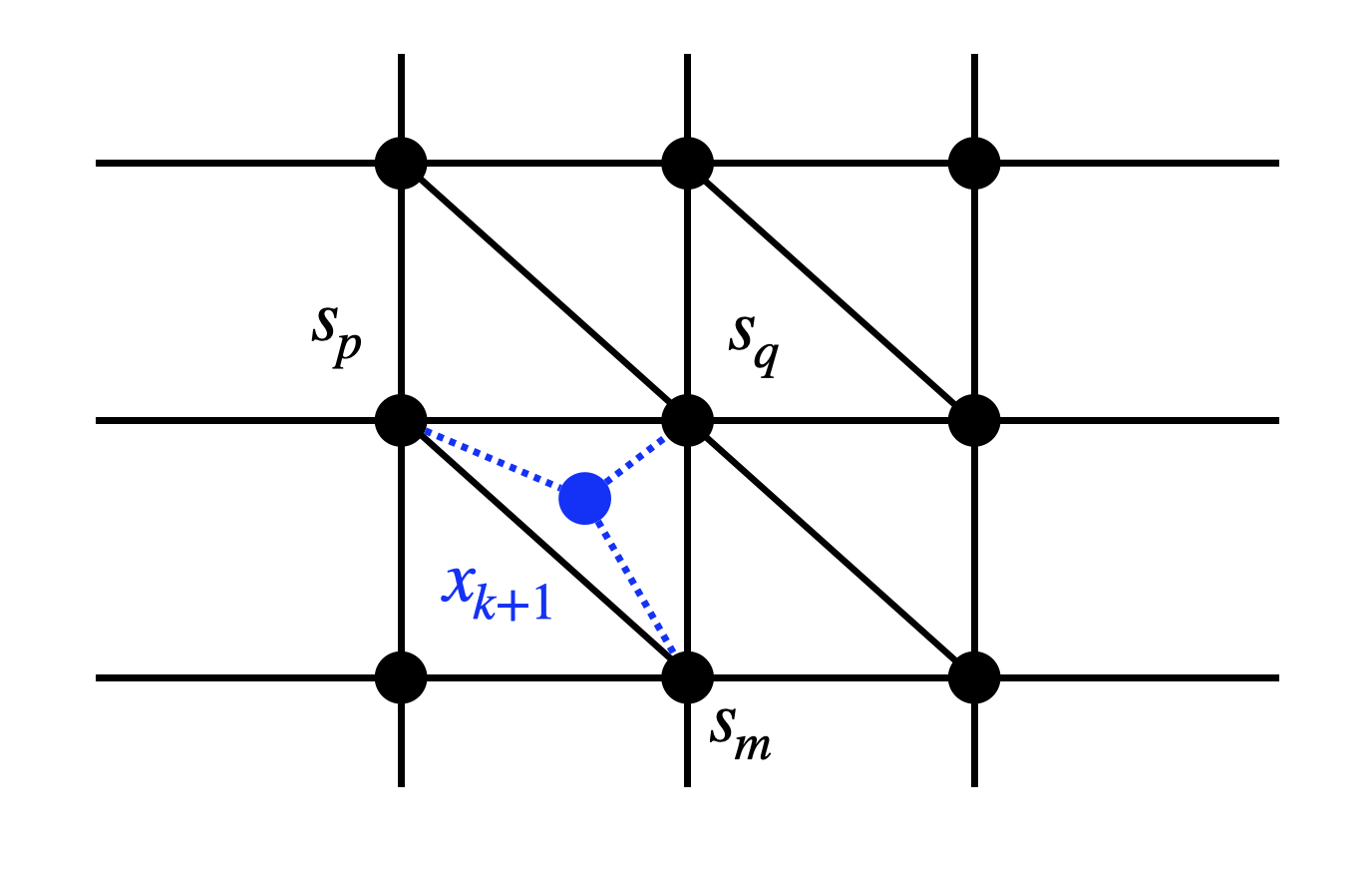
Figure 2.5: Barycentric Interpolation.

Nevertheless, $x_{k+1}$ will lie inside a triangle with vertices $s_p, s_q, s_m$. We will now try to write $x_{k+1}$ using the vertices, that is, to find three numbers $\lambda_p, \lambda_q, \lambda_m$ such that $$\lambda_p, \lambda_q, \lambda_m \geq 0, \quad \lambda_p + \lambda_q + \lambda_m = 1, \quad x_{k+1} = \lambda_p s_p + \lambda_q s_q + \lambda_m s_m.$$ $\lambda_p,\lambda_q,\lambda_m$ are called the barycentric coordinates of $x_{k+1}$ in the triangle formed by $s_p,s_q,s_m$. With the barycentric coordinates, we will assign the transition matrix $$P(x_{k+1}=s_p \mid x_k,u_k) = \lambda_p, \quad P(x_{k+1}=s_q \mid x_k,u_k) = \lambda_q, \quad P(x_{k+1}=s_m \mid x_k,u_k) = \lambda_m.$$

Let us apply value iteration with barycentric interpolation to the simple pendulum.

Example 2.3 (Value Iteration with Barycentric Interpolation on A Simple Pendulum) Consider the continuous-time pendulum dynamics in (2.15) that is already shifted such that $z=0$ corresponds to the upright position. With time discretization $h$, we can write the discrete-time dynamics as $$z_{k+1} = \dot{z}_k \cdot h + z_k = f'(z_k,u_k) \cdot h + z_k.$$ We are interested in solving the optimal control problem $$J(z_0) = \min_{u_k} \left\{ \sum_{k=0}^{\infty} \gamma^k g(x_k,u_k) \right\},$$ where the running cost is simply $$g(x_k,u_k) = x_k^T x_k + u_k^2.$$

We will use the parameters $m=1,g=9.8,l=1,b=0.1$, and assume the control is bounded in $[-4.9,4.9]$.

We want to compute the optimal cost-to-go in the range $z_1 \in [-\pi,\pi]$ and $z_2 \in [-\pi,\pi]$. We discretize both $z_1$ and $z_2$ using $N$ points, leading to $N^2$ points in the state space. We also discretize $u$ using $N$ points.

Applying value iteration with $\gamma=0.9$ and $N=50$, we obtain the optimal cost-to-go in Fig. 2.6. The value iteration converges in $277$ iterations.

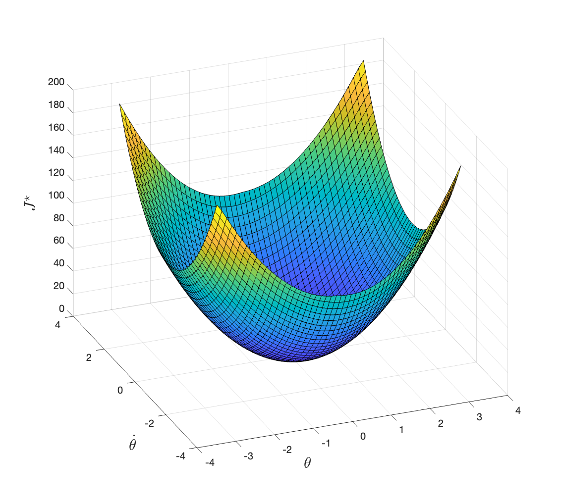
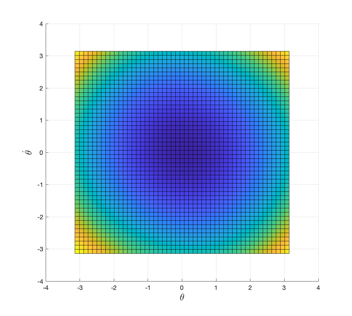
Figure 2.6: Optimal cost-to-go with discount factor 0.9.

Applying value iteration with $\gamma=0.99$ and $N=50$, we obtain the optimal cost-to-go in Fig. 2.7. The value iteration converges in $2910$ iterations.

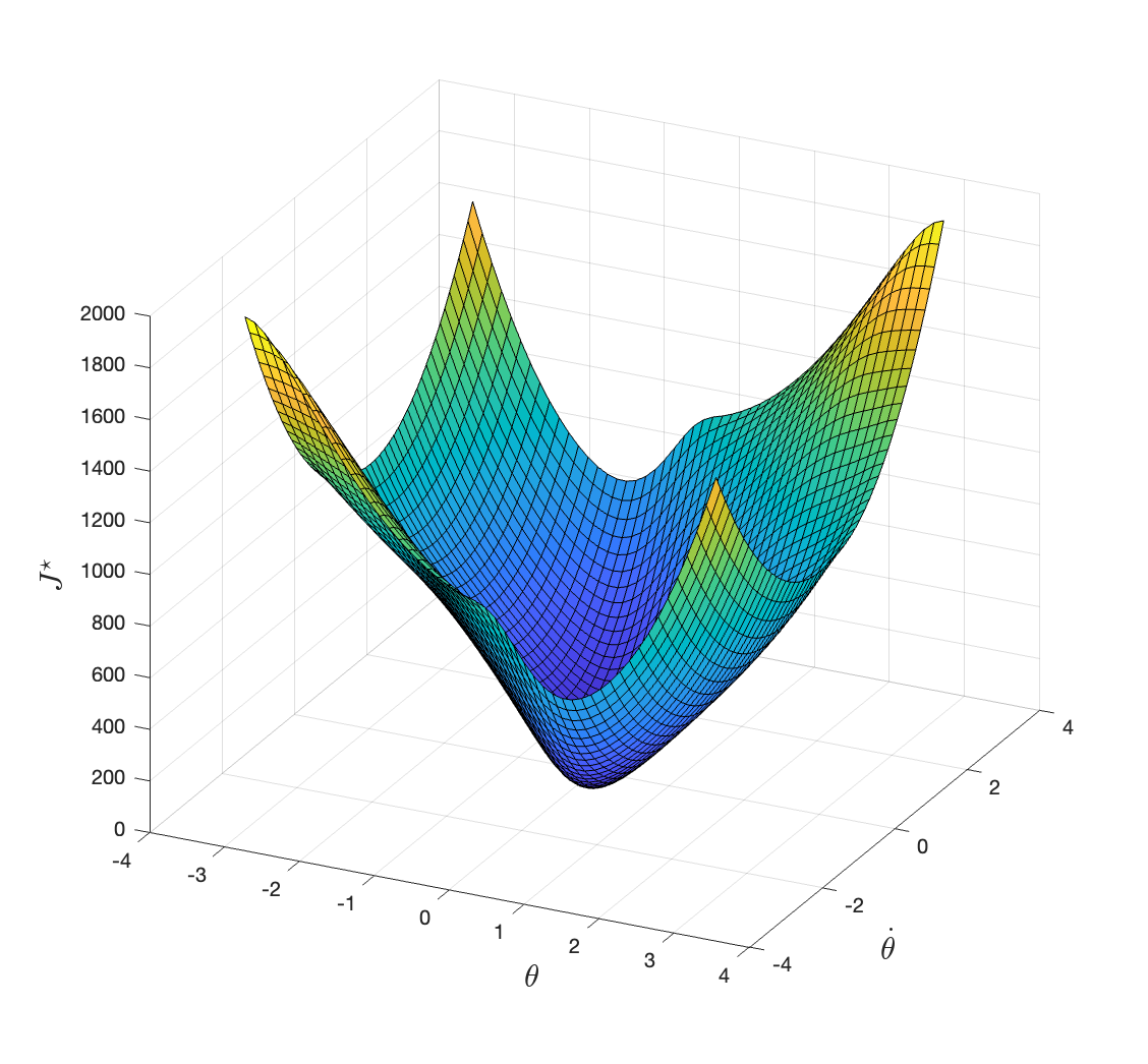
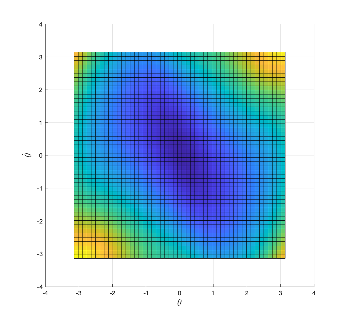
Figure 2.7: Optimal cost-to-go with discount factor 0.99.

Applying value iteration with $\gamma=0.999$ and $N=50$, we obtain the optimal cost-to-go in Fig. 2.8. The value iteration converges in $28850$ iterations.

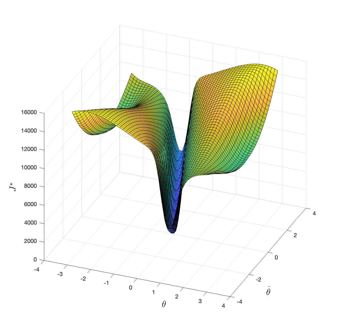
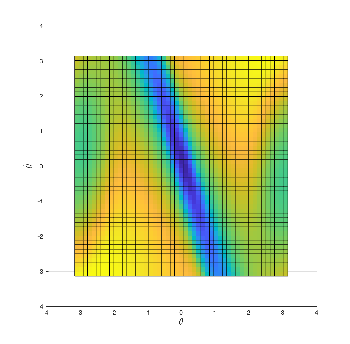
Figure 2.8: Optimal cost-to-go with discount factor 0.999.

You can find the Matlab code here.

References

Agarwal, Alekh, Nan Jiang, Sham M Kakade, and Wen Sun. 2022. “Reinforcement Learning: Theory and Algorithms.” CS Dept., UW Seattle, Seattle, WA, USA, Tech. Rep 32.

Arnold, William F, and Alan J Laub. 1984. “Generalized Eigenproblem Algorithms and Software for Algebraic Riccati Equations.” Proceedings of the IEEE 72 (12): 1746–54.

———. 2012. Dynamic Programming and Optimal Control: Volume i. Vol. 1. Athena scientific.

---

3. One can show that the matrix $I - \gamma P^\pi$ is indeed invertible, see Corollary 1.5 in (Agarwal et al. 2022).↩︎