Chapter 1 Markov Decision Process

Optimal control (OC) and reinforcement learning (RL) address the problem of making optimal decisions in the presence of a dynamic environment.

In optimal control, this dynamic environment is often referred to as a plant or a dynamical system.
In reinforcement learning, it is modeled as a Markov decision process (MDP).

The goal in both fields is to evaluate and design decision-making strategies that optimize long-term performance:

RL typically frames this as maximizing a long-term reward.
OC often formulates it as minimizing a long-term cost.

The emphasis on long-term evaluation is crucial. Because the environment evolves over time, decisions that appear beneficial in the short term may lead to poor long-term outcomes and thus be suboptimal.

With this motivation, we now formalize the framework of Markov Decision Processes (MDPs), which are discrete-time stochastic dynamical systems.

1.1 Finite-Horizon MDP

We begin with finite-horizon MDPs and introduce infinite-horizon MDPs in the following section. An abstract definition of the finite-horizon case will be presented first, followed by illustrative examples.

A finite-horizon MDP is given by the following tuple: \[ \mathcal{M} = (\mathcal{S}, \mathcal{A}, P, R, T), \] where

\(\mathcal{S}\): state space (set of all possible states)
\(\mathcal{A}\): action space (set of all possible actions)
\(P(s' \mid s, a)\): probability of transitioning to state \(s'\) from state \(s\) under action \(a\) (i.e., dynamics)
\(R(s,a)\): reward of taking action \(a\) in state \(s\)
\(T\): horizon, a positive integer

For now, let us assume both the state space and the action space are discrete and have a finite number of elements. In particular, denote the number of elements in \(\mathcal{S}\) as \(|\mathcal{S}|\), and the number of elements in \(\mathcal{A}\) as \(|\mathcal{A}|\). This is also referred to as a tabular MDP.

Policy. Decision-making in MDPs is represented by policies. A policy is a function that, given any state, outputs a distribution of actions: \(\pi: \mathcal{S} \mapsto \Delta(\mathcal{A})\). That is, \(\pi(a \mid s)\) returns the probability of taking action \(a\) in state \(s\). In finite-horizon MDPs, we consider a tuple of policies: \[\begin{equation} \pi = (\pi_0, \dots, \pi_t, \dots, \pi_{T-1}), \tag{1.1} \end{equation}\] where each \(\pi_t\) denotes the policy at step \(t \in [0,T-1]\).

Trajectory and Return. Given an initial state \(s_0 \in \mathcal{S}\) and a policy \(\pi\), the MDP will evolve as

Start at state \(s_0\)
Take action \(a_0 \sim \pi_0(a \mid s_0)\) following policy \(\pi_0\)
Collect reward \(r_0 = R(s_0, a_0)\) (assume \(R\) is deterministic)
Transition to state \(s_1 \sim P(s' \mid s_0, a_0)\) following the dynamics
Go to step 2 and continue until reaching state \(s_T\)

This evolution generates a trajectory of states, actions, and rewards: \[ \tau = (s_0, a_0, r_0, s_1, a_1, r_1,\dots, s_{T-1}, a_{T-1}, r_{T-1}, s_T). \] The cumulative reward of this trajectory is \(g_0 = \sum_{t=0}^{T-1} r_t\), which is called the return of the trajectory. Clearly, \(g_0\) is a random variable due to the stochasticity of both the policy and the dynamics. Similarly, if the state at time \(t\) is \(s_t\), we denote: \[ g_t = r_t + \dots + r_{T-1} \] as the return of the policy starting at \(s_t\).

1.1.1 Value Functions

State-Value Function. Given a policy \(\pi\) as in (1.1), which states are preferable at time \(t\)? The (time-indexed) state-value function assigns to each \(s\in\mathcal{S}\) the expected return from \(t\) onward when starting in \(s\) and following \(\pi\) thereafter. Formally, define \[\begin{equation} V_t^\pi(s) := \mathbb{E} \left[g_t \mid s_t=s\right] = \mathbb{E} \left[\sum_{i=t}^{T-1} R(s_i,a_i) \middle| s_t=s,a_i\sim \pi_i(\cdot\mid s_i), s_{i+1}\sim P(\cdot\mid s_i,a_i)\right]. \tag{1.2} \end{equation}\] The expectation is over the randomness induced by both the policy and the dynamics. Thus, if \(V_t^\pi(s_1)>V_t^\pi(s_2)\), then at time \(t\) under policy \(\pi\) it is better in expectation to be in \(s_1\) than in \(s_2\) because the former yields a larger expected return.

\(V^{\pi}_t(s)\): given policy \(\pi\), how good is it to start in state \(s\) at time \(t\)?

Action-Value Function. Similarly, the action-value function assigns to each state-action pair \((s,a)\in\mathcal{S}\times\mathcal{A}\) the expected return obtained by starting in state \(s\), taking action \(a\) first, and then following policy \(\pi\) thereafter: \[\begin{equation} \begin{split} Q_t^\pi(s,a) := & \mathbb{E} \left[R(s,a) + g_{t+1} \mid s_{t+1} \sim P(\cdot \mid s,a)\right] \\ = & \mathbb{E} \left[R(s,a) + \sum_{i=t+1}^{T-1} R(s_i, a_i) \middle| s_{t+1} \sim P(\cdot \mid s,a) \right]. \end{split} \tag{1.3} \end{equation}\] The key distinction is that the action-value function evaluates the return when the first action may deviate from policy \(\pi\), whereas the state-value function assumes strict adherence to \(\pi\). This flexibility makes the action-value function central to improving \(\pi\), since it reveals whether alternative actions can yield higher returns.

\(Q^{\pi}_t(s,a)\): At time \(t\), how good is it to take action \(a\) in state \(s\), then follow the policy \(\pi\)?

It is easy to verify that the state-value function and the action-value function satisfy: \[\begin{align} V_t^{\pi}(s) & = \sum_{a \in \mathcal{A}} \pi_t(a \mid s) Q_t^{\pi}(s,a), \tag{1.4} \\ Q_t^{\pi}(s,a) & = R(s,a) + \sum_{s' \in \mathcal{S}} P(s' \mid s, a) V^{\pi}_{t+1} (s'). \tag{1.5} \end{align}\]

From these two equations, we can derive the Bellman Consistency equations.

Proposition 1.1 (Bellman Consistency (Finite Horizon)) The state-value function \(V^{\pi}_t(\cdot)\) in (1.2) satisfies the following recursion: \[\begin{equation} \begin{split} V^{\pi}_t(s) & = \sum_{a \in \mathcal{A}} \pi_t(a\mid s) \left( R(s,a) + \sum_{s' \in \mathcal{S}} P(s' \mid s, a) V^{\pi}_{t+1} (s') \right) \\ & =: \mathbb{E}_{a \sim \pi_t(\cdot \mid s)} \left[ R(s, a) + \mathbb{E}_{s' \sim P(\cdot \mid s, a)} [V^{\pi}_{t+1}(s')] \right]. \end{split} \tag{1.6} \end{equation}\]

Similarly, the action-value function \(Q^{\pi}_t(s,a)\) in (1.3) satisfies the following recursion: \[\begin{equation} \begin{split} Q^{\pi}_t (s, a) & = R(s,a) + \sum_{s' \in \mathcal{S}} P(s' \mid s, a) \left( \sum_{a' \in \mathcal{A}} \pi_{t+1}(a' \mid s') Q^{\pi}_{t+1}(s', a')\right) \\ & =: R(s, a) + \mathbb{E}_{s' \sim P(\cdot \mid s, a)} \left[\mathbb{E}_{a' \sim \pi_{t+1}(\cdot \mid s')} [Q^{\pi}_{t+1}(s', a')] \right]. \end{split} \tag{1.7} \end{equation}\]

1.1.2 Policy Evaluation

The Bellman consistency result in Proposition 1.1 is fundamental because it directly yields an algorithm for evaluating a given policy \(\pi\)—that is, for computing its state-value and action-value functions—provided the transition dynamics of the MDP are known.

Policy evaluation for the state-value function proceeds as follows:

Initialization: set \(V^{\pi}_T(s) = 0\) for all \(s \in \mathcal{S}\).
Backward recursion: for \(t = T-1, T-2, \dots, 0\), update each \(s \in \mathcal{S}\) by \[ V^{\pi}_{t}(s) = \mathbb{E}_{a \sim \pi_t(\cdot \mid s)} \left[ R(s, a) + \mathbb{E}_{s' \sim P(\cdot \mid s, a)} \big[ V^{\pi}_{t+1}(s') \big] \right]. \]

Similarly, policy evaluation for the action-value function is given by:

Initialization: set \(Q^{\pi}_T(s,a) = 0\) for all \(s \in \mathcal{S}, a \in \mathcal{A}\).
Backward recursion: for \(t = T-1, T-2, \dots, 0\), update each \((s,a) \in \mathcal{S}\times\mathcal{A}\) by \[ Q^{\pi}_t(s,a) = R(s, a) + \mathbb{E}_{s' \sim P(\cdot \mid s, a)} \left[ \mathbb{E}_{a' \sim \pi_{t+1}(\cdot \mid s')} \big[ Q^{\pi}_{t+1}(s', a') \big] \right]. \]

The essential feature of this algorithm is its backward-in-time recursion: the value functions are first set at the terminal horizon \(T\), and then propagated backward step by step through the Bellman consistency equations.

Example 1.1 (MDP, Transition Graph, and Policy Evaluation) It is often useful to visualize small MDPs as transition graphs, where states are represented by nodes and actions are represented by directed edges connecting those nodes.

As a simple illustrative example, consider a robot navigating on a two-state grid. At each step, the robot can either Stay in its current state or Move to the other state. This finite-horizon MDP is fully specified by the tuple of states, actions, transition dynamics, rewards, and horizon:

States: \(\mathcal{S} = \{\alpha, \beta \}\)
Actions: \(\mathcal{A} = \{\text{Move} , \text{Stay} \}\)
Transition dynamics: we can specify the transition dynamics in the following table

State \(s\)	Action \(a\)	Next State \(s'\)	Probability \(P(s' \mid s, a)\)
\(\alpha\)	Stay	\(\alpha\)	1
\(\alpha\)	Move	\(\beta\)	1
\(\beta\)	Stay	\(\beta\)	1
\(\beta\)	Move	\(\alpha\)	1

Reward: \(R(s,a)=1\) if \(a = \text{Move}\) and \(R(s,a)=0\) if \(a = \text{Stay}\)
Horizon: \(T=2\).

This MDP can be represented by the transition graph in Fig. 1.1. Note that for this MDP, the transition dynamics is deterministic. We will see a stochastic MDP soon.

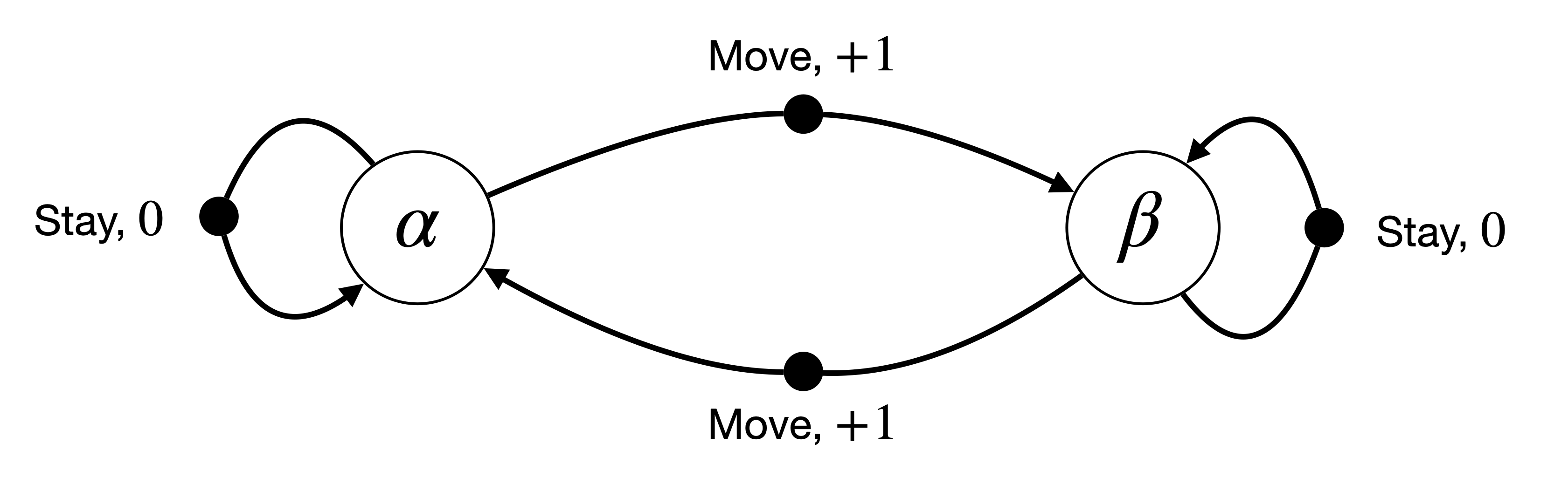
Figure 1.1: A Simple Transition Graph.

At time \(t=0\), if the robot starts at \(s_0 = \alpha\), first chooses action \(a_0 = \text{Move}\), and then chooses action \(a_1 = \text{Stay}\), the resulting trajectory is \[ \tau = (\alpha, \text{Move}, +1, \beta, \text{Stay}, 0, \beta). \] The return of this trajectory is: \[ g_0 = +1 + 0 = +1. \]

Policy Evaluation. Given a policy \[\begin{equation} \pi = (\pi_0, \pi_1), \quad \pi_0(a \mid s) = \begin{cases} 0.5 & a = \text{Move} \\ 0.5 & a = \text{Stay} \end{cases}, \quad \pi_1( a \mid s) = \begin{cases} 0.8 & a = \text{Move} \\ 0.2 & a = \text{Stay} \end{cases}. \end{equation}\] We can use the Bellman consistency equations to compute the state-value function. We first initialize: \[ V^{\pi}_2 = \begin{bmatrix} 0 \\ 0 \end{bmatrix}, \] where the first row contains the value at \(s = \alpha\) and the second row contains the value at \(s = \beta\). We then perform the backward recursion for \(t=1\). For \(s = \alpha\), we have \[\begin{equation} V^{\pi}_1(\alpha) = \begin{bmatrix} \pi_1(\text{Move} \mid \alpha) \\ \pi_1(\text{Stay} \mid \alpha) \end{bmatrix}^{\top} \begin{bmatrix} R(\alpha, \text{Move}) + V^{\pi}_2(\beta) \\ R(\alpha, \text{Stay}) + V^{\pi}_2(\alpha) \end{bmatrix} = \begin{bmatrix} 0.8 \\ 0.2 \end{bmatrix}^{\top} \begin{bmatrix} 1 \\ 0 \end{bmatrix} = 0.8 \end{equation}\] For \(s = \beta\), we have \[\begin{equation} V^{\pi}_1(\beta) = \begin{bmatrix} \pi_1(\text{Move} \mid \beta) \\ \pi_1(\text{Stay} \mid \beta) \end{bmatrix}^{\top} \begin{bmatrix} R(\beta, \text{Move}) + V^{\pi}_2(\alpha) \\ R(\beta, \text{Stay}) + V^{\pi}_2(\beta) \end{bmatrix} = \begin{bmatrix} 0.8 \\ 0.2 \end{bmatrix}^{\top} \begin{bmatrix} 1 \\ 0 \end{bmatrix} = 0.8. \end{equation}\] Therefore, we have \[ V^{\pi}_1 = \begin{bmatrix} 0.8 \\ 0.8 \end{bmatrix}. \] We then proceed to the backward recursion for \(t=0\): \[\begin{align} V_0^{\pi}(\alpha) & = \begin{bmatrix} \pi_0(\text{Move} \mid \alpha) \\ \pi_0(\text{Stay} \mid \alpha) \end{bmatrix}^{\top} \begin{bmatrix} R(\alpha, \text{Move}) + V^{\pi}_1(\beta) \\ R(\alpha, \text{Stay}) + V^{\pi}_1(\alpha) \end{bmatrix} = \begin{bmatrix} 0.5 \\ 0.5 \end{bmatrix}^{\top} \begin{bmatrix} 1.8 \\ 0.8 \end{bmatrix} = 1.3. \\ V_0^{\pi}(\beta) & = \begin{bmatrix} \pi_0(\text{Move} \mid \beta) \\ \pi_0(\text{Stay} \mid \beta) \end{bmatrix}^{\top} \begin{bmatrix} R(\beta, \text{Move}) + V^{\pi}_0(\alpha) \\ R(\beta, \text{Stay}) + V^{\pi}_0(\beta) \end{bmatrix} = \begin{bmatrix} 0.5 \\ 0.5 \end{bmatrix}^{\top} \begin{bmatrix} 1.8 \\ 0.8 \end{bmatrix} = 1.3. \end{align}\] Therefore, the state-value function at \(t=0\) is \[ V^{\pi}_0 = \begin{bmatrix} 1.3 \\ 1.3 \end{bmatrix}. \] You are encouraged to carry out the similar calculations for the action-value function.

The toy example was small enough to carry out policy evaluation by hand; in realistic MDPs, we will need the help from computers.

Consider now an MDP whose transition graph is shown in Fig. 1.2. This example is adapted from here.

Figure 1.2: Hangover Transition Graph.

This MDP has six states: \[ \mathcal{S} = \{\text{Hangover}, \text{Sleep}, \text{More Sleep}, \text{Visit Lecture}, \text{Study}, \text{Pass Exam} \}, \] and two actions: \[ \mathcal{A} = \{\text{Lazy}, \text{Productive} \}. \] The stochastic transition dynamics are labeled in the transition graph. For example, at state “Hangover”, taking action “Productive” will lead to state “Visit Lecture” with probability \(0.3\) and state “Hangover” with probability \(0.7\). The rewards of the MDP are defined as: \[ R(s,a) = \begin{cases} +1 & s = \text{Pass Exam} \\ -1 & \text{otherwise}. \end{cases}. \]

Policy Evaluation. Consider a time-invariant random policy \[ \pi = \{\pi_0,\dots,\pi_{T-1} \}, \quad \pi_t(a \mid s) = \begin{cases} \alpha & a = \text{Lazy} \\ 1 - \alpha & a = \text{Productive} \end{cases}, \] that takes “Lazy” with probability \(\alpha\) and “Productive” with probability \(1-\alpha\).

The following Python code performs policy evaluation for this MDP, with \(T=10\) and \(\alpha = 0.4\).

# Finite-horizon policy evaluation for the Hangover MDP

from collections import defaultdict
from typing import Dict, List, Tuple

State = str
Action = str

# --- MDP spec ---------------------------------------------------------------

S: List[State] = [
    "Hangover", "Sleep", "More Sleep", "Visit Lecture", "Study", "Pass Exam"
]
A: List[Action] = ["Lazy", "Productive"]

# P[s, a] -> list of (s_next, prob)
P: Dict[Tuple[State, Action], List[Tuple[State, float]]] = {
    # Hangover
    ("Hangover", "Lazy"):       [("Sleep", 1.0)],
    ("Hangover", "Productive"): [("Visit Lecture", 0.3), ("Hangover", 0.7)],

    # Sleep
    ("Sleep", "Lazy"):          [("More Sleep", 1.0)],
    ("Sleep", "Productive"):    [("Visit Lecture", 0.6), ("More Sleep", 0.4)],

    # More Sleep
    ("More Sleep", "Lazy"):       [("More Sleep", 1.0)],
    ("More Sleep", "Productive"): [("Study", 0.5), ("More Sleep", 0.5)],

    # Visit Lecture
    ("Visit Lecture", "Lazy"):       [("Study", 0.8), ("Pass Exam", 0.2)],
    ("Visit Lecture", "Productive"): [("Study", 1.0)],

    # Study
    ("Study", "Lazy"):         [("More Sleep", 1.0)],
    ("Study", "Productive"):   [("Pass Exam", 0.9), ("Study", 0.1)],

    # Pass Exam (absorbing)
    ("Pass Exam", "Lazy"):       [("Pass Exam", 1.0)],
    ("Pass Exam", "Productive"): [("Pass Exam", 1.0)],
}

def R(s: State, a: Action) -> float:
    """Reward: +1 in Pass Exam, -1 otherwise."""
    return 1.0 if s == "Pass Exam" else -1.0

# --- Policy: time-invariant, state-independent ------------------------------

def pi(a: Action, s: State, alpha: float) -> float:
    """pi(a|s): Lazy with prob alpha, Productive with prob 1-alpha."""
    return alpha if a == "Lazy" else (1.0 - alpha)

# --- Policy evaluation -------------------------------------------------------

def policy_evaluation(T: int, alpha: float):
    """
    Compute {V_t(s)} and {Q_t(s,a)} for t=0..T with terminal condition V_T = Q_T = 0.
    Returns:
        V: Dict[int, Dict[State, float]]
        Q: Dict[int, Dict[Tuple[State, Action], float]]
    """
    assert T >= 0
    # sanity: probabilities sum to 1 for each (s,a)
    for key, rows in P.items():
        total = sum(p for _, p in rows)
        if abs(total - 1.0) > 1e-9:
            raise ValueError(f"Probabilities for {key} sum to {total}, not 1.")

    V: Dict[int, Dict[State, float]] = defaultdict(dict)
    Q: Dict[int, Dict[Tuple[State, Action], float]] = defaultdict(dict)

    # Terminal boundary
    for s in S:
        V[T][s] = 0.0
        for a in A:
            Q[T][(s, a)] = 0.0

    # Backward recursion
    for t in range(T - 1, -1, -1):
        for s in S:
            # First compute Q_t(s,a)
            for a in A:
                exp_next = sum(p * V[t + 1][s_next] for s_next, p in P[(s, a)])
                Q[t][(s, a)] = R(s, a) + exp_next
            # Then V_t(s) = E_{a~pi}[Q_t(s,a)]
            V[t][s] = sum(pi(a, s, alpha) * Q[t][(s, a)] for a in A)

    return V, Q

# --- Example run -------------------------------------------------------------

if __name__ == "__main__":
    T = 10        # horizon
    alpha = 0.4  # probability of choosing Lazy
    V, Q = policy_evaluation(T=T, alpha=alpha)

    # Print V_0
    print(f"V_0(s) with T={T}, alpha={alpha}:")
    for s in S:
        print(f"  {s:13s}: {V[0][s]: .3f}")

The code returns the following state values at \(t=0\): \[\begin{equation} V^{\pi}_0 = \begin{bmatrix} -3.582 \\ -2.306 \\ -2.180 \\ 1.757 \\ 2.939 \\ 10 \end{bmatrix}, \tag{1.8} \end{equation}\] where the ordering of the states follows that defined in \(\mathcal{S}\).

You can find the code here.

1.1.3 Principle of Optimality

Every policy \(\pi\) induces a value function \(V_0^{\pi}\) that can be evaluated by policy evaluation (assuming the transition dynamics are known). The goal of reinforcement learning is to find an optimal policy that maximizes the value function with respect to a given initial state distribution: \[\begin{equation} V^\star_0 = \max_{\pi}\; \mathbb{E}_{s_0 \sim \mu(\cdot)} \big[ V_0^{\pi}(s_0) \big], \tag{1.9} \end{equation}\] where we have used the superscript “\(\star\)” to denote the optimality of the value function. \(V^\star_0\) is often known as the optimal value function.

At first glance, (1.9) appears daunting: a naive approach would enumerate all stochastic policies \(\pi\), evaluate their value functions, and select the best. A central result in reinforcement learning and optimal control—rooted in the principle of optimality—is that the optimal value functions satisfy a Bellman-style recursion, analogous to Proposition 1.1. This Bellman optimality recursion enables backward computation of the optimal value functions without enumerating policies.

Theorem 1.1 (Bellman Optimality (Finite Horizon, State-Value)) Consider a finite-horizon MDP \(\mathcal{M}=(\mathcal{S},\mathcal{A},P,R,T)\) with finite state and action sets and bounded rewards. Define the optimal value functions \(\{V_t^\star\}_{t=0}^{T}\) by the following Bellman optimality recursion \[\begin{equation} \begin{split} V_T^\star(s)& \equiv 0, \\ V_t^\star(s)& = \max_{a\in\mathcal{A}}\Big\{ R(s,a)\;+\;\sum_{s'\in\mathcal{S}} P(s'\mid s,a)\,V_{t+1}^\star(s')\Big\},\ t=T-1,\ldots,0. \end{split} \tag{1.10} \end{equation}\] Then, the optimal value functions are optimal in the sense of statewise dominance: \[\begin{equation} V_t^{\star}(s)\;\ge\; V_t^{\pi}(s) \quad\text{for all policies }\pi,\; s\in\mathcal{S},\; t=0,\ldots,T. \tag{1.11} \end{equation}\]

Moreover, the deterministic policy \(\pi^\star=(\pi^\star_0,\ldots,\pi^\star_{T-1})\) with \[\begin{equation} \begin{split} \pi_t^\star(s)\;\in\;\arg\max_{a\in\mathcal{A}} \Big\{ R(s,a)\;+\;\sum_{s'\in\mathcal{S}} P(s'\mid s,a)\,V_{t+1}^\star(s')\Big\}, \\ \text{for any } s\in\mathcal{S},\; t=0,\dots,T-1 \end{split} \tag{1.12} \end{equation}\] is optimal, where ties can be broken by any fixed rule.

Proof. We first show that the value functions defined by the Bellman optimality recursion (1.10) are optimal in the sense that they dominate the value functions of any other policy. The proof proceeds by backward induction.

Base case (\(t=T\)). For every \(s\in\mathcal{S}\), \[ V^\star_T(s)\;=\;0\;=\;V_T^{\pi}(s), \] so \(V^\star_T(s)\ge V_T^{\pi}(s)\) holds trivially.

Inductive step. Assume \(V^\star_{t+1}(s)\ge V^{\pi}_{t+1}(s)\) for all \(s\in\mathcal{S}\). Then, for any \(s\in\mathcal{S}\), \[\begin{align*} V_t^{\pi}(s) &= \sum_{a\in\mathcal{A}} \pi_t(a\mid s)\!\left(R(s,a)+\sum_{s'\in\mathcal{S}} P(s'\mid s,a)\,V_{t+1}^{\pi}(s')\right) \\ &\le \sum_{a\in\mathcal{A}} \pi_t(a\mid s)\!\left(R(s,a)+\sum_{s'\in\mathcal{S}} P(s'\mid s,a)\,V_{t+1}^{\star}(s')\right) \\ &\le \max_{a\in\mathcal{A}} \left(R(s,a)+\sum_{s'\in\mathcal{S}} P(s'\mid s,a)\,V_{t+1}^{\star}(s')\right) \;=\; V_t^\star(s), \end{align*}\] where the first inequality uses the induction hypothesis and the second uses that an expectation is bounded above by a maximum. Hence \(V_t^\star(s)\ge V_t^{\pi}(s)\) for all \(s\), completing the induction. Therefore, \(\{V_t^\star\}_{t=0}^T\) dominates the value functions attainable by any policy.

Next, we show that \(\{V_t^\star\}\) is attainable by some policy. Since \(\mathcal{A}\) is finite (tabular setting), the maximizer in the Bellman optimality operator exists for every \((t,s)\); thus we can define a (deterministic) greedy policy \[ \pi_t^\star(s)\;\in\;\arg\max_{a\in\mathcal{A}} \Big\{ R(s,a)+\sum_{s'\in\mathcal{S}} P(s'\mid s,a)\,V_{t+1}^\star(s') \Big\}. \] A simple backward induction then shows \(V_t^{\pi^\star}(s)=V_t^\star(s)\) for all \(t\) and \(s\): at \(t=T\) both are \(0\), and if \(V_{t+1}^{\pi^\star}=V_{t+1}^\star\), then by construction of \(\pi_t^\star\) the Bellman equality yields \(V_t^{\pi^\star}=V_t^\star\). Consequently, the optimal value functions are achieved by the greedy (deterministic) policy \(\pi^\star\).

Corollary 1.1 (Bellman Optimality (Finite Horizon, Action-Value)) Given the optimal (state-)value functions \(V^{\star}_{t},t=0,\dots,T\), define the optimal action-value function \[\begin{equation} Q_t^\star(s,a)\;=\;R(s,a)+\sum_{s'\in\mathcal{S}} P(s'\mid s,a)\,V_{t+1}^\star(s'), \quad t=0,\dots,T-1. \tag{1.13} \end{equation}\]

Then we have \[\begin{equation} V_t^\star(s)=\max_{a\in\mathcal{A}} Q_t^\star(s,a),\qquad \pi_t^\star(s)\in\arg\max_{a\in\mathcal{A}} Q_t^\star(s,a). \tag{1.14} \end{equation}\]

The optimal action-value functions satisfy: \[\begin{equation} \begin{split} Q_T^\star(s,a) & \equiv 0,\\ Q_t^\star(s,a) & = R(s,a) \;+\; \mathbb{E}_{s'\sim P(\cdot\mid s,a)} \!\left[ \max_{a'\in\mathcal{A}} Q_{t+1}^\star(s',a') \right], \quad t=T-1,\ldots,0. \end{split} \tag{1.15} \end{equation}\]

1.1.4 Dynamic Programming

The principle of optimality in Theorem 1.1 yields a constructive procedure to compute the optimal value functions and an associated deterministic optimal policy. This backward-induction procedure is the dynamic programming (DP) algorithm.

Dynamic programming (finite horizon).

Initialization. Set \(V_T^\star(s) = 0\) for all \(s \in \mathcal{S}\).
Backward recursion. For \(t = T-1, T-2, \dots, 0\):
- Optimal value: for each \(s \in \mathcal{S}\), \[ V_t^\star(s) = \max_{a \in \mathcal{A}} \left\{ R(s,a) + \mathbb{E}_{s' \sim P(\cdot \mid s,a)} \big[ V_{t+1}^\star(s') \big] \right\}. \]
- Greedy policy (deterministic): for each \(s \in \mathcal{S}\), \[ \pi_t^\star(s) \in \arg\max_{a \in \mathcal{A}} \left\{ R(s,a) + \mathbb{E}_{s' \sim P(\cdot \mid s,a)} \big[ V_{t+1}^\star(s') \big] \right\}. \]

Exercise 1.1 How does dynamic programming look like when applied to the action-value function?

Exercise 1.2 What is the computational complexity of dynamic programming?

Let us try dynamic programming for the Hangover MDP presented before.

Example 1.2 (Dynamic Programming for Hangover MDP) Consider the Hangover MDP defined by the transition graph shown in Fig. 1.2. With slight modification to the policy evaluation code, we can find the optimal value functions and optimal policies.

# Dynamic programming (finite-horizon optimal control) for the Hangover MDP

from collections import defaultdict
from typing import Dict, List, Tuple

State = str
Action = str

# --- MDP spec ---------------------------------------------------------------

S: List[State] = [
    "Hangover", "Sleep", "More Sleep", "Visit Lecture", "Study", "Pass Exam"
]
A: List[Action] = ["Lazy", "Productive"]

# P[s, a] -> list of (s_next, prob)
P: Dict[Tuple[State, Action], List[Tuple[State, float]]] = {
    # Hangover
    ("Hangover", "Lazy"):       [("Sleep", 1.0)],
    ("Hangover", "Productive"): [("Visit Lecture", 0.3), ("Hangover", 0.7)],

    # Sleep
    ("Sleep", "Lazy"):          [("More Sleep", 1.0)],
    ("Sleep", "Productive"):    [("Visit Lecture", 0.6), ("More Sleep", 0.4)],

    # More Sleep
    ("More Sleep", "Lazy"):       [("More Sleep", 1.0)],
    ("More Sleep", "Productive"): [("Study", 0.5), ("More Sleep", 0.5)],

    # Visit Lecture
    ("Visit Lecture", "Lazy"):       [("Study", 0.8), ("Pass Exam", 0.2)],
    ("Visit Lecture", "Productive"): [("Study", 1.0)],

    # Study
    ("Study", "Lazy"):         [("More Sleep", 1.0)],
    ("Study", "Productive"):   [("Pass Exam", 0.9), ("Study", 0.1)],

    # Pass Exam (absorbing)
    ("Pass Exam", "Lazy"):       [("Pass Exam", 1.0)],
    ("Pass Exam", "Productive"): [("Pass Exam", 1.0)],
}

def R(s: State, a: Action) -> float:
    """Reward: +1 in Pass Exam, -1 otherwise."""
    return 1.0 if s == "Pass Exam" else -1.0

# --- Dynamic programming (Bellman optimality) -------------------------------

def dynamic_programming(T: int):
    """
    Compute optimal finite-horizon tables:
      - V[t][s] = V_t^*(s)
      - Q[t][(s,a)] = Q_t^*(s,a)
      - PI[t][s] = optimal action at (t,s)
    with terminal condition V_T^* = 0.
    """
    assert T >= 0

    # sanity: probabilities sum to 1 for each (s,a)
    for key, rows in P.items():
        total = sum(p for _, p in rows)
        if abs(total - 1.0) > 1e-9:
            raise ValueError(f"Probabilities for {key} sum to {total}, not 1.")

    V: Dict[int, Dict[State, float]] = defaultdict(dict)
    Q: Dict[int, Dict[Tuple[State, Action], float]] = defaultdict(dict)
    PI: Dict[int, Dict[State, Action]] = defaultdict(dict)

    # Terminal boundary
    for s in S:
        V[T][s] = 0.0
        for a in A:
            Q[T][(s, a)] = 0.0

    # Backward recursion (Bellman optimality)
    for t in range(T - 1, -1, -1):
        for s in S:
            # compute Q*_t(s,a)
            for a in A:
                exp_next = sum(p * V[t + 1][s_next] for s_next, p in P[(s, a)])
                Q[t][(s, a)] = R(s, a) + exp_next

            # greedy action and optimal value
            # tie-breaking is deterministic by the order in A
            best_a = max(A, key=lambda a: Q[t][(s, a)])
            PI[t][s] = best_a
            V[t][s] = Q[t][(s, best_a)]

    return V, Q, PI

# --- Example run -------------------------------------------------------------

if __name__ == "__main__":
    T = 10  # horizon
    V, Q, PI = dynamic_programming(T=T)

    print(f"Optimal V_0(s) with T={T}:")
    for s in S:
        print(f"  {s:13s}: {V[0][s]: .3f}")

    print("\nGreedy policy at t=0:")
    for s in S:
        print(f"  {s:13s}: {PI[0][s]}")

    print("\nAction value at t=0:")
    for s in S:
        print(f"  {s:13s}: {Q[0][s, A[0]]: .3f}, {Q[0][s, A[1]]: .3f}")

The optimal value function at \(t=0\) is: \[\begin{equation} V^\star_0 = \begin{bmatrix} 1.259 \\ 3.251 \\ 3.787 \\ 6.222 \\ 7.778 \\ 10 \end{bmatrix}. \tag{1.16} \end{equation}\] Clearly, the optimal value function dominates the value function shown in (1.8) of the random policy at every state.

The optimal actions at \(t=0\) are: \[\begin{equation} \begin{split} \text{Hangover} & : \text{Lazy} \\ \text{Sleep} & : \text{Productive} \\ \text{More Sleep} & : \text{Productive} \\ \text{Visit Lecture} & : \text{Lazy} \\ \text{Study} & : \text{Productive} \\ \text{Pass Exam} & : \text{Lazy} \end{split}. \end{equation}\]

You can play with the code here.

1.2 Infinite-Horizon MDP

In a finite-horizon MDP, the horizon \(T\) must be specified in advance in order to carry out policy evaluation and dynamic programming. The finite horizon naturally provides a terminal condition, which serves as the boundary condition that allows backward recursion to proceed.

In many practical applications, however, the horizon \(T\) is not well defined or is difficult to determine. In such cases, it is often more natural and convenient to adopt the infinite-horizon MDP formulation.

An infinite-horizon MDP is given by the following tuple: \[ \mathcal{M} = (\mathcal{S}, \mathcal{A}, P, R, \gamma), \] where \(\mathcal{S}\), \(\mathcal{A}\), \(P\), and \(R\) are the same as defined before in a finite-horizon MDP. We still restrict ourselves to the tabular MDP setup where \(\mathcal{S}\) and \(\mathcal{A}\) both have a finite number of elements.

The key difference between the finite-horizon and infinite-horizon formulations is that the fixed horizon \(T\) is replaced by a discount factor \(\gamma \in [0,1)\). This discount factor weights future rewards less heavily than immediate rewards, as we will see shortly.

Stationary Policy. In an infinite-horizon MDP, we focus on stationary policies \(\pi: \mathcal{S} \mapsto \Delta(\mathcal{A})\), where \(\pi(a \mid s)\) denotes the probability of taking action \(a\) in state \(s\).

In contrast, in a finite-horizon MDP we considered a tuple of \(T\) policies (see (1.1)), where each \(\pi_t\) could vary with time (i.e., policies were non-stationary).

Intuitively, in the infinite-horizon setting, it suffices to consider stationary policies because the decision-making problem at time \(t\) is equivalent to the problem at time \(t + k\) for any \(k \in \mathbb{N}\), as both face the same infinite horizon.

Trajectory and Return. Given an initial state \(s_0 \in \mathcal{S}\) and a stationary policy \(\pi\), the MDP will evolve as

Start at state \(s_0\)
Take action \(a_0 \sim \pi(\cdot \mid s_0)\) following policy \(\pi\)
Collect reward \(r_0 = R(s_0, a_0)\)
Transition to state \(s_1 \sim P(s' \mid s_0, a_0)\) following the dynamics
Go to step 2 and continue forever

This process generates a trajectory of states, actions, and rewards: \[ \tau = (s_0, a_0, r_0, s_1, a_1, r_1, \dots). \]

The return of a trajectory is defined as \[ g_0 = r_0 + \gamma r_1 + \gamma^2 r_2 + \dots = \sum_{t=0}^{\infty} \gamma^t r_t. \]

Here, the discount factor \(\gamma\) plays a key role: it progressively reduces the weight of rewards received further in the future, making them less influential as \(t\) increases.

1.2.1 Value Functions

Similar to the case of finite-horizon MDP, we can define the state-value function and the action-value function associated with a policy \(\pi\).

State-Value Function. The value of a state \(s \in \mathcal{S}\) under policy \(\pi\) is the expected discounted return obtained when starting from \(s\) at time \(0\): \[\begin{equation} V^{\pi}(s) := \mathbb{E}\left[ \sum_{t=0}^{\infty} \gamma^t R(s_t, a_t) \,\middle|\, s_0 = s, a_t \sim \pi(\cdot \mid s_t), s_{t+1} \sim P(\cdot \mid s_t, a_t) \right]. \tag{1.17} \end{equation}\]

Action-Value Function. The value of a state-action pair \((s,a) \in \mathcal{S} \times \mathcal{A}\) under policy \(\pi\) is the expected discounted return obtained by first taking action \(a\) in state \(s\), and then following policy \(\pi\) thereafter: \[\begin{equation} Q^{\pi}(s,a) := \mathbb{E} \left[ \sum_{t=0}^{\infty} \gamma^t R(s_t, a_t) \,\middle|\, s_0 = s, a_0 = a, a_t \sim \pi(\cdot \mid s_t), s_{t+1} \sim P(\cdot \mid s_t, a_t) \right]. \tag{1.18} \end{equation}\]

Note that a nice feature of having a discount factor \(\gamma \in [0,1)\) is that both the state-value and the action-value functions are guaranteed to be bounded even if the horizon is unbounded (assuming the reward function is bounded).

We can verify the state-value function and the action value function satisfy the following relationship: \[\begin{align} V^{\pi}(s) &= \sum_{a \in \mathcal{A}} \pi(a \mid s) Q^{\pi}(s,a) \tag{1.19}\\ Q^{\pi}(s,a) & = R(s,a) + \gamma \sum_{s' \in \mathcal{S}} P(s' \mid s, a) V^{\pi}(s'). \tag{1.20} \end{align}\]

Combining these two equations, we arrive at the Bellman consistency result for infinite-horizon MDP.

Proposition 1.2 (Bellman Consistency (Infinite Horizon)) The state-value function \(V^{\pi}\) in (1.17) satisfies the following recursion: \[\begin{equation} \begin{split} V^{\pi} (s) & = \sum_{a \in \mathcal{A}} \pi (a\mid s) \left( R(s,a) + \gamma \sum_{s' \in \mathcal{S}} P(s' \mid s, a) V^{\pi} (s') \right) \\ & =: \mathbb{E}_{a \sim \pi(\cdot \mid s)} \left[ R(s, a) + \gamma \mathbb{E}_{s' \sim P(\cdot \mid s, a)} [V^{\pi}(s')] \right]. \end{split} \tag{1.21} \end{equation}\]

Similarly, the action-value function \(Q^{\pi}(s,a)\) in (1.18) satisfies the following recursion: \[\begin{equation} \begin{split} Q^{\pi} (s, a) & = R(s,a) + \gamma \sum_{s' \in \mathcal{S}} P(s' \mid s, a) \left( \sum_{a' \in \mathcal{A}} \pi(a' \mid s') Q^{\pi}(s', a')\right) \\ & =: R(s, a) + \gamma \mathbb{E}_{s' \sim P(\cdot \mid s, a)} \left[\mathbb{E}_{a' \sim \pi(\cdot \mid s')} [Q^{\pi}(s', a')] \right]. \end{split} \tag{1.22} \end{equation}\]

1.2.2 Policy Evaluation

Given a policy \(\pi\), how can we compute its associated state-value and action-value functions?

Finite-horizon case. We initialize the terminal value function \(V_T^{\pi}(s) = 0\) for every \(s \in \mathcal{S}\), and then apply the Bellman Consistency result (Proposition 1.1) to perform backward recursion.
Infinite-horizon case. The Bellman Consistency result (Proposition 1.2) takes a different form and does not provide the same simple recipe for backward recursion.

System of Linear Equations. A closer look at the Bellman Consistency equation (1.21) for the state-value function shows that it defines a square system of linear equations. Specifically, the value function \(V^{\pi}\) can be represented as a vector with \(|\mathcal{S}|\) variables, and (1.21) provides \(|\mathcal{S}|\) linear equations over these variables.
Thus, one way to compute the state-value function is to set up this linear system and solve it. However, doing so typically requires matrix inversion or factorization, which can be computationally expensive.

The same reasoning applies to the action-value function \(Q^{\pi}\), which can be represented as a vector of \(|\mathcal{S}||\mathcal{A}|\) variables constrained by \(|\mathcal{S}||\mathcal{A}|\) linear equations.

The following proposition states that, instead of solving a linear system of equations, one can use a globally convergent iterative scheme, one that is very much like the policy evaluation algorithm for the finite-horizon MDP, to evaluate the state-value function associated with a policy \(\pi\).

Proposition 1.3 (Policy Evaluation (Infinite Horizon, State-Value)) Consider an infinite-horizon MDP \(\mathcal{M}=(\mathcal{S},\mathcal{A},P,R,\gamma)\). Fix a policy \(\pi\) and consider the iterative scheme for the state-value function: \[\begin{equation} V_{k+1}(s) \;\; \gets \;\; \sum_{a \in \mathcal{A}} \pi(a \mid s) \left[ R(s,a) + \gamma \sum_{s' \in \mathcal{S}} P(s' \mid s,a) V_k(s') \right], \quad \forall s \in \mathcal{S}. \tag{1.23} \end{equation}\]

Then, starting from any initialization \(V_0 \in \mathbb{R}^{|\mathcal{S}|}\), the sequence \(\{V_k\}\) converges to the unique fixed point \(V^{\pi}\), the state-value function associated with policy \(\pi\).

Proof. To prove the convergence of the policy evaluation algorithm, we shall introduce the notion of a Bellman operator.

Bellman Operator. Any value function \(V(s)\) can be interpreted as a vector in \(\mathbb{R}^{|\mathcal{S}|}\) (recall we are in the tabular MDP case). Given any value function \(V \in \mathbb{R}^{|\mathcal{S}|}\), and a policy \(\pi\), define the Bellman operator associated with \(\pi\) as \(T^{\pi}: \mathbb{R}^{|\mathcal{S}|} \mapsto \mathbb{R}^{|\mathcal{S}|}\): \[\begin{equation} (T^{\pi} V)(s) := \sum_{a \in \mathcal{A}} \pi(a \mid s) \left[ R(s,a) + \gamma \sum_{s' \in \mathcal{S}} P(s' \mid s,a) V(s') \right]. \tag{1.24} \end{equation}\]

We claim that \(T^{\pi}\) has two important properties.

Monotonicity. If \(V \leq W\) (i.e., \(V(s) \leq W(s)\) for any \(s \in \mathcal{S}\)), then \(T^{\pi} V \leq T^{\pi}W\). To see this, observe that \[\begin{align*} (T^{\pi}V)(s) - (T^\pi W)(s) &= \sum_{a} \pi(a \mid s) \left(\gamma \sum_{s'} P(s' \mid s, a) (V(s') - W(s')) \right) \\ & = \gamma \mathbb{E}_{a \sim \pi(\cdot \mid s), s' \sim P(\cdot \mid s,a)}[V(s') - W(s')]. \end{align*}\] Therefore, if \(V(s') - W(s') \leq 0\) for any \(s' \in \mathcal{S}\), then \(T^{\pi}V \leq T^{\pi} W\).
\(\gamma\)-Contraction. For any value function \(V \in \mathbb{R}^{|\mathcal{S}|}\), define the \(\ell_{\infty}\) norm (sup norm) as \[ \Vert V \Vert_{\infty} = \max_{s \in \mathcal{S}} |V(s)|. \]

We claim that the Bellman operator \(T^{\pi}\) is a \(\gamma\)-contraction in the sup norm, i.e., \[\begin{equation} \Vert T^\pi V - T^\pi W \Vert_{\infty} \leq \gamma \Vert V - W \Vert_{\infty}, \quad \forall V, W \in \mathbb{R}^{|\mathcal{S}|}. \tag{1.25} \end{equation}\] To prove this, observe that for any \(s \in \mathcal{S}\), we have: \[\begin{align*} |(T^\pi V)(s) - (T^\pi W)(s)| &= \left| \sum_a \pi(a|s)\,\gamma \sum_{s'} P(s'|s,a)\big(V(s') - W(s')\big) \right| \\ &\le \gamma \sum_a \pi(a|s)\sum_{s'} P(s'|s,a)\,|V(s') - W(s')| \\ &\le \gamma \|V - W\|_\infty \sum_a \pi(a|s)\sum_{s'} P(s'|s,a) \\ &= \gamma \|V - W\|_\infty. \end{align*}\]

Taking the maximum over \(s\) gives \[ \|T^\pi V - T^\pi W\|_\infty \le \gamma \|V - W\|_\infty, \] so \(T^\pi\) is a \(\gamma\)-contraction in the sup norm.

With the Bellman operator defined, we observe that the value function of \(\pi\), denoted \(V^{\pi}\) in (1.21), is a fixed point of \(T^{\pi}\). That is to say \(V^{\pi}\) satisfies: \[ T^{\pi} V^{\pi} = V^{\pi}. \] In other words, \(V^{\pi}\) is fixed (remains unchanged) under the Bellman operator.

Since \(T^{\pi}\) is a \(\gamma\)-contraction, by the Banach Fixed-Point Theorem, we know that there exists a unique fixed point to \(T^{\pi}\), which is \(V^{\pi}\). Moreover, since \[ \Vert V_{k} - V^{\pi} \Vert_{\infty} = \Vert T^{\pi} V_{k-1} - T^{\pi} V^{\pi} \Vert_{\infty} \leq \gamma \Vert V_{k-1} - V^{\pi} \Vert_{\infty}, \] we can deduce the rate of convergence \[ \Vert V_{k} - V^{\pi} \Vert_{\infty} \leq \gamma^{k} \Vert V_0 - V^{\pi} \Vert_{\infty}. \] Therefore, policy evaluation globally converges from any initialization \(V_0\) at a linear rate of \(\gamma\).

We have a similar policy evaluation algorithm for the action-value function.

Proposition 1.4 (Policy Evaluation (Infinite Horizon, Action-Value)) Fix a policy \(\pi\). Consider the iterative scheme on \(Q:\mathcal{S}\times\mathcal{A}\to\mathbb{R}\): \[\begin{equation} \begin{split} Q_{k+1}(s,a) \;\gets\; R(s,a) \;+\; \gamma \sum_{s'\in\mathcal{S}} P(s'\mid s,a)\!\left(\sum_{a'\in\mathcal{A}} \pi(a'\mid s')\, Q_k(s',a')\right), \\ \forall (s,a)\in\mathcal{S}\times\mathcal{A}. \end{split} \tag{1.26} \end{equation}\] Then, for any initialization \(Q_0\), the sequence \(\{Q_k\}\) converges to the unique fixed point \(Q^{\pi}\), the action-value function associated with policy \(\pi\).

Proof. Define the Bellman operator on action-values \[ (T^{\pi}Q)(s,a) := R(s,a) + \gamma \sum_{s'} P(s'\mid s,a)\Big(\sum_{a'} \pi(a'\mid s')\, Q(s',a')\Big). \] \(T^{\pi}\) is a \(\gamma\)-contraction in the sup-norm on \(\mathbb{R}^{|\mathcal{S}||\mathcal{A}|}\); hence by the Banach fixed-point theorem, global convergence holds regardless of initialization.

Let us apply policy evaluation to an infinite-horizon MDP.

Example 1.3 (Policy Evaluation for Inverted Pendulum)

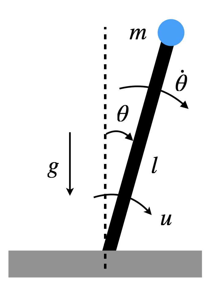
Figure 1.3: Inverted Pendulum.

We consider the inverted pendulum with state \(s=(\theta, \dot\theta)\) and action (torque) \(a = u\), as visualized in Fig. 1.3. Our goal is to swing up the pendulum from any initial state to the upright position \(s = (0,0)\).

Continuous-Time Dynamics. The continuous-time dynamics of the inverted pendulum is \[ \ddot{\theta} \;=\; \frac{g}{l}\sin(\theta) \;+\; \frac{1}{ml^2}u \;-\; c\,\dot{\theta}, \] where \(m > 0\) is the mass of the pendulum, \(l > 0\) is the length of the pole, \(c > 0\) is the damping coefficient, and \(g\) is the gravitational constant.

Discretization (Euler). With timestep \(\Delta t\), we obtain the following discrete-time dynamics: \[\begin{equation} \begin{split} \theta_{k+1} &= \theta_k + \Delta t \, \dot{\theta}_k, \\ \dot{\theta}_{k+1} &= \dot{\theta}_k + \Delta t \Big(\tfrac{g}{l}\sin(\theta_k) + \tfrac{1}{ml^2}u_k - c\,\dot{\theta}_k\Big). \end{split} \tag{1.27} \end{equation}\]

We wrap angles to \([-\pi,\pi]\) via \(\operatorname{wrap}(\theta)=\mathrm{atan2}(\sin\theta,\cos\theta)\).

Tabular MDP. We convert the discrete-time dynamics into a tabular MDP.

State grid. \(\theta \in [-\pi,\pi]\), \(\dot\theta \in [-\pi,\pi]\) on uniform grids: \[ \mathcal{S}=\{\;(\theta_i,\dot\theta_j)\;:\; i=1,\dots,N_\theta,\; j=1, \dots, N_{\dot\theta}\;\}. \]
Action grid. \(u \in [-mgl/2, mgl/2]\) on \(N_u\) uniform points: \[ \mathcal{A}=\{u_\ell:\ell=1,\dots,N_u\}. \]
Stochastic transition kernel (nearest-3 interpolation). From a grid point \(s=(\theta_i,\dot\theta_j)\) and an action \(u_\ell\), compute the next continuous state \(s^+ = (\theta^+,\dot\theta^+)\) via the discrete-time dynamics in (1.27). If \(s^+\notin\mathcal{S}\), choose the three closest grid states \(\{s^{(1)},s^{(2)},s^{(3)}\}\) by Euclidean distance in \((\theta,\dot\theta)\) and assign probabilities \[ p_r \propto \frac{1}{\|s^+ - s^{(r)}\|_2 + \varepsilon},\quad r=1,2,3, \qquad \sum_r p_r=1, \] so nearer grid points receive higher probability (use a small \(\varepsilon>0\) to avoid division by zero).
Reward. A quadratic shaping penalty around the upright equilibrium: \[ R(s,a) = -\Big(\theta^2 + 0.1\,\dot\theta^2 + 0.01\,u^2\Big). \]
Discount. \(\gamma \in [0,1)\). We obtain a discounted, infinite-horizon, tabular MDP.

Policy. For policy evaluation, consider \(\pi(a\mid s)\) be uniform over the discretized actions, i.e., a random policy.

Policy Evaluation. The following python script performs policy evaluation.

import numpy as np
import matplotlib.pyplot as plt

# ----- Physical & MDP parameters -----
g, l, m, c = 9.81, 1.0, 1.0, 0.1
dt = 0.05
gamma = 0.97
eps = 1e-8

# Grids
N_theta = 41
N_thetadot = 41
N_u = 21

theta_grid = np.linspace(-np.pi, np.pi, N_theta)
thetadot_grid = np.linspace(-np.pi, np.pi, N_thetadot)
u_max = 0.5 * m * g * l
u_grid = np.linspace(-u_max, u_max, N_u)

# Helpers to index/unwrap
def wrap_angle(x):
    return np.arctan2(np.sin(x), np.cos(x))

def state_index(i, j):
    return i * N_thetadot + j

def index_to_state(idx):
    i = idx // N_thetadot
    j = idx % N_thetadot
    return theta_grid[i], thetadot_grid[j]

S = N_theta * N_thetadot
A = N_u

# ----- Dynamics step (continuous -> one Euler step) -----
def step_euler(theta, thetadot, u):
    theta_next = wrap_angle(theta + dt * thetadot)
    thetadot_next = thetadot + dt * ((g/l) * np.sin(theta) + (1/(m*l*l))*u - c*thetadot)
    # clip angular velocity to grid range (bounded MDP)
    thetadot_next = np.clip(thetadot_next, thetadot_grid[0], thetadot_grid[-1])
    return theta_next, thetadot_next

# ----- Find 3 nearest grid states and probability weights (inverse-distance) -----
# Pre-compute all grid points for fast nearest neighbor search
grid_pts = np.stack(np.meshgrid(theta_grid, thetadot_grid, indexing='ij'), axis=-1).reshape(-1, 2)

def nearest3_probs(theta_next, thetadot_next):
    x = np.array([theta_next, thetadot_next])
    dists = np.linalg.norm(grid_pts - x[None, :], axis=1)
    nn_idx = np.argpartition(dists, 3)[:3]  # three smallest (unordered)
    # sort those 3 by distance for stability
    nn_idx = nn_idx[np.argsort(dists[nn_idx])]
    d = dists[nn_idx]
    w = 1.0 / (d + eps)
    p = w / w.sum()
    return nn_idx.astype(int), p

# ----- Reward -----
def reward(theta, thetadot, u):
    return -(theta**2 + 0.1*thetadot**2 + 0.01*u**2)

# ----- Build tabular MDP: R[s,a] and sparse P[s,a,3] -----
R = np.zeros((S, A))
NS_idx = np.zeros((S, A, 3), dtype=int)   # next-state indices (3 nearest)
NS_prob = np.zeros((S, A, 3))            # their probabilities

for i, th in enumerate(theta_grid):
    for j, thd in enumerate(thetadot_grid):
        s = state_index(i, j)
        for a, u in enumerate(u_grid):
            # reward at current (s,a)
            R[s, a] = reward(th, thd, u)
            # next continuous state
            th_n, thd_n = step_euler(th, thd, u)
            # map to 3 nearest grid states
            nn_idx, p = nearest3_probs(th_n, thd_n)
            NS_idx[s, a, :] = nn_idx
            NS_prob[s, a, :] = p

# ----- Fixed policy: uniform over actions -----
Pi = np.full((S, A), 1.0 / A)

# ----- Iterative policy evaluation -----
V = np.zeros(S)  # initialization (any vector works)
tol = 1e-6
max_iters = 10000

for k in range(max_iters):
    V_new = np.zeros_like(V)
    # Compute Bellman update: V_{k+1}(s) = sum_a Pi(s,a)[ R(s,a) + gamma * sum_j P(s,a,j) V_k(ns_j) ]
    # First, expected next V for each (s,a)
    EV_next = (NS_prob * V[NS_idx]).sum(axis=2)  # shape: (S, A)
    # Then expectation over actions under Pi
    V_new = (Pi * (R + gamma * EV_next)).sum(axis=1)  # shape: (S,)
    # Check convergence
    if np.max(np.abs(V_new - V)) < tol:
        V = V_new
        print(f"Converged in {k+1} iterations (sup-norm change < {tol}).")
        break
    V = V_new
else:
    print(f"Reached max_iters={max_iters} without meeting tolerance {tol}.")

V_grid = V.reshape(N_theta, N_thetadot)

# V_grid: shape (N_theta, N_thetadot)
# theta_grid, thetadot_grid already defined
fig, ax = plt.subplots(figsize=(7,5), dpi=120)
im = ax.imshow(
    V_grid,
    origin="lower",
    extent=[thetadot_grid.min(), thetadot_grid.max(),
            theta_grid.min(), theta_grid.max()],
    aspect="auto",
    cmap="viridis"  # any matplotlib colormap, e.g., "plasma", "inferno"
)
cbar = fig.colorbar(im, ax=ax)
cbar.set_label(r"$V^\pi(\theta,\dot{\theta})$")

ax.set_xlabel(r"$\dot{\theta}$")
ax.set_ylabel(r"$\theta$")
ax.set_title(r"State-value $V^\pi$ (tabular policy evaluation)")

plt.tight_layout()
plt.show()

Running the code, it shows that policy evaluation converges in 518 iterations under tolerance \(10^{-6}\).

Fig. 1.4 plots the value function over the state grid.

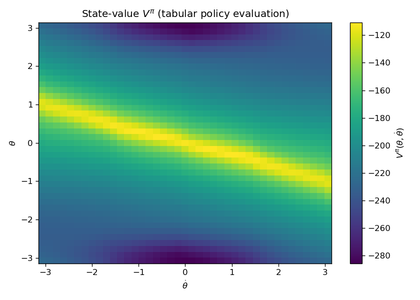
Figure 1.4: Value Function from Policy Evaluation.

You can play with the code here.

1.2.3 Principle of Optimality

In an infinite-horizon MDP, our goal is to find the optimal policy that maximizes the expected long-term discounted return: \[ V^\star := \max_{\pi} \mathbb{E}_{s \sim \mu(\cdot)} [V^\pi(s)], \] where \(\mu\) is a given initial distribution. We call \(V^\star\) the optimal value function.

Given a policy \(\pi\) and its associated value function \(V^\pi\), how do we know if the policy is already optimal?

Theorem 1.2 (Bellman Optimality (Infinite Horizon)) For an infinite-horizon MDP with discount factor \(\gamma \in [0,1)\), the optimal state-value function \(V^\star(s)\) satisfies the Bellman optimality equation \[\begin{equation} V^\star(s) \;=\; \max_{a \in \mathcal{A}} \Big[\, R(s,a) + \gamma \sum_{s' \in \mathcal{S}} P(s' \mid s,a)\, V^\star(s') \,\Big]. \tag{1.28} \end{equation}\]

Define the optimal action-value function as \[\begin{equation} Q^\star(s,a) = R(s,a) + \gamma \sum_{s' \in \mathcal{S}} P(s' \mid s, a) V^\star(s'). \tag{1.29} \end{equation}\] We have that \(Q^\star(s,a)\) satisfies \[\begin{equation} Q^\star(s,a) \;=\; R(s,a) + \gamma \sum_{s' \in \mathcal{S}} P(s' \mid s,a)\, \left[\max_{a' \in \mathcal{A}} Q^\star(s',a') \right]. \tag{1.30} \end{equation}\]

Moreover, any greedy policy with respect to \(V^\star\) (equivalently, to \(Q^\star\)) is optimal: \[\begin{equation} \begin{split} \pi^\star(s) & \in \arg\max_{a \in \mathcal{A}} \Big[\, R(s,a) + \gamma \sum_{s'} P(s' \mid s,a)\, V^\star(s') \,\Big] \quad\Longleftrightarrow\quad \\ \pi^\star(s) & \in \arg\max_{a \in \mathcal{A}} Q^\star(s,a). \end{split} \tag{1.31} \end{equation}\]

Proof. We will first show that \(V^\star\) has statewise dominance over all other policies, and then show that \(V^\star\) can be attained by the greedy policy.

Claim. For any discounted MDP with \(\gamma \in [0,1)\) and any policy \(\pi\), \[ V^\star(s) \;\ge\; V^{\pi}(s)\qquad \forall s\in\mathcal{S}, \] where \(V^\star\) is the unique solution of the Bellman optimality equation and \(V^\pi\) solves the Bellman consistency equation for \(\pi\).

Proof via Bellman Operators. Define the Bellman operators \[ (T^\pi V)(s) := \sum_{a}\pi(a\mid s)\Big[ R(s,a)+\gamma \sum_{s'} P(s'\mid s,a)V(s') \Big], \] \[ (T^\star V)(s) := \max_{a}\Big[ R(s,a)+\gamma \sum_{s'} P(s'\mid s,a)V(s') \Big]. \]

Key facts:

(Monotonicity) If \(V \ge W\) componentwise, then \(T^\pi V \ge T^\pi W\) and \(T^\star V \ge T^\star W\).
(Dominance of \(T^*\)) For any \(V\) and any \(\pi\), \[ T^\star V \;\ge\; T^\pi V \] because the max over actions is at least the \(\pi\)-weighted average.
(Fixed points) \(V^\pi = T^\pi V^\pi\) and \(V^\star = T^\star V^\star\).
(Contraction) Each \(T^\pi\) and \(T^\star\) is a \(\gamma\)-contraction in the sup-norm; hence their fixed points are unique.

Now start from \(V^\pi\). Using (2), \[ V^\pi = T^\pi V^\pi \;\le\; T^\star V^\pi. \] Applying \(T^\star\) repeatedly and using (1), \[ V^\pi \;\le\; T^\star V^\pi \;\le\; (T^\star)^2 V^\pi \;\le\; \cdots \] The sequence \((T^\star)^k V^\pi\) converges (by contraction) to the unique fixed point of \(T^\star\), namely \(V^\star\). Taking limits preserves the inequality, yielding \(V^\pi \le V^\star\) statewise.

The Bellman optimality condition tells us, if a policy \(\pi\) is already greedy with respect to its value function \(V^\pi\), then \(\pi\) is the optimal policy and \(V^\pi\) is the optimal value function.

In the next, we introduce two algorithms that can guarantee finding the optimal policy and the optimal value function.

The first algorithm, policy iteration (PI), iterates over the space of policies; while the second algorithm, value iteration (VI), iterates over the space of value functions.

1.2.4 Policy Improvement

The policy evaluation algorithm enables us to compute the value functions associated with a given policy \(\pi\). The next result, known as the Policy Improvement Lemma, shows that once we have \(V^{\pi}\), constructing a greedy policy with respect to \(V^{\pi}\) guarantees performance that is at least as good as \(\pi\), and strictly better in some states unless \(\pi\) is already greedy with respect to \(V^{\pi}\).

Lemma 1.1 (Policy Improvement) Let \(\pi\) be any policy and let \(V^{\pi}\) be its state-value function.
Define a new policy \(\pi'\) such that for each state \(s\), \[ \pi'(s) \in \arg\max_{a \in \mathcal{A}} \Big[ R(s,a) + \gamma \sum_{s'} P(s' \mid s,a) V^{\pi}(s') \Big]. \]

Then for all states \(s \in \mathcal{S}\), \[ V^{\pi'}(s) \;\ge\; V^{\pi}(s). \] Moreover, the inequality is strict for some state \(s\) unless \(\pi\) is already greedy with respect to \(V^\pi\) (which implies optimality).

Proof. Let \(V^{\pi}\) be the value function of a policy \(\pi\), and define a new (possibly stochastic) policy \(\pi'\) that is greedy w.r.t. \(V^{\pi}\): \[ \pi'(\cdot \mid s) \in \arg\max_{\mu \in \Delta(\mathcal{A})} \sum_{a}\mu(a)\Big[ R(s,a) + \gamma \sum_{s'} P(s'\mid s,a)\, V^{\pi}(s')\Big]. \] Define the Bellman operators \[\begin{align*} (T^{\pi}V)(s) & := \sum_a \pi(a\mid s)\Big[R(s,a)+\gamma\sum_{s'}P(s'\mid s,a)V(s')\Big],\\ (T^{\pi'}V)(s) & := \sum_a \pi'(a\mid s)\Big[\cdots\Big]. \end{align*}\]

Step 1: One-step improvement at \(V^{\pi}\). By greediness of \(\pi'\) w.r.t. \(V^{\pi}\), \[ (T^{\pi'} V^{\pi})(s) = \max_{\mu}\sum_a \mu(a)\Big[R(s,a)+\gamma\sum_{s'}P(s'\mid s,a)V^{\pi}(s')\Big] \;\;\ge\;\; (T^{\pi} V^{\pi})(s) = V^{\pi}(s), \] for all \(s\). Hence \[\begin{equation} T^{\pi'} V^{\pi} \;\ge\; V^{\pi}\quad\text{(componentwise).} \tag{1.32} \end{equation}\]

Step 2: Monotonicity + contraction yield global improvement. The operator \(T^{\pi'}\) is monotone (order-preserving) and a \(\gamma\)-contraction in the sup-norm.
Apply \(T^{\pi'}\) repeatedly to both sides of (1.32): \[ (T^{\pi'})^k V^{\pi} \;\ge\; (T^{\pi'})^{k-1} V^{\pi} \;\ge\; \cdots \;\ge\; V^{\pi},\qquad k=1,2,\dots \] By contraction, \((T^{\pi'})^k V^{\pi} \to V^{\pi'}\), the unique fixed point of \(T^{\pi'}\).
Taking limits preserves the inequality, so \[ V^{\pi'} \;\ge\; V^{\pi}\quad\text{statewise.} \]

Strict improvement condition. If there exists a state \(s\) such that \[ (T^{\pi'} V^{\pi})(s) \;>\; V^{\pi}(s), \] then by monotonicity we have a strict increase at that state after one iteration, and the limit remains strictly larger at that state (or at any state that can reach it with positive probability under \(\pi'\)).
This happens precisely when \(\pi'\) selects, with positive probability, an action \(a\) for which \[ Q^{\pi}(s,a)=R(s,a) + \gamma \sum_{s'} P(s'\mid s,a)\, V^{\pi}(s') \;>\; V^{\pi}(s), \] i.e., when \(\pi\) was not already greedy (optimal) at \(s\).

1.2.5 Policy Iteration

The policy improvement lemma and the principle of optimality, combined together, leads to the first algorithm that guarantees convergence to an optimal policy. This algorithm is called policy iteration.

Theorem 1.3 (Convergence of Policy Iteration) Consider a discounted MDP with finite state and action sets and \(\gamma\in[0,1)\). Let \(\{\pi_k\}_{k\ge0}\) be the sequence produced by Policy Iteration (PI):

Policy evaluation: compute \(V^{\pi_k}\) such that \(V^{\pi_k}=T^{\pi_k}V^{\pi_k}\).
Policy improvement: choose \(\pi_{k+1}\) greedy w.r.t. \(V^{\pi_k}\): \[ \pi_{k+1}(s) \in \arg\max_{a}\Big[ R(s,a)+\gamma\sum_{s'}P(s'|s,a)\,V^{\pi_k}(s')\Big]. \]

Then:

\(V^{\pi_{k+1}} \ge V^{\pi_k}\) componentwise, and the inequality is strict for some state unless \(\pi_{k+1}=\pi_k\).
If \(\pi_{k+1}=\pi_k\), then \(V^{\pi_k}\) satisfies the Bellman optimality equation; hence \(\pi_k\) is optimal and \(V^{\pi_k}=V^*\).
Because the number of stationary policies is finite, PI terminates in finitely many iterations at an optimal policy \(\pi^*\) with value \(V^*\).
\(\Vert V^{\pi_{k+1}} - V^\star \Vert_{\infty} \leq \gamma \Vert V^{\pi_k} - V^\star \Vert_{\infty}\), for any \(k\) (i.e., contraction).

Proof. By the policy improvement lemma, we have \[ V^{\pi_{k+1}} \geq V^{\pi_k}. \] By monotonicity of the Bellman operator \(T^{\pi_{k+1}}\), we have \[ V^{\pi_{k+1}} = T^{\pi_{k+1}} V^{\pi_{k+1}} \geq T^{\pi_{k+1}} V^{\pi_k}. \] By definition of the Bellman optimality operator, we have \[ T^{\pi_{k+1}} V^{\pi_k} = T^\star V^{\pi_k}. \] Therefore, \[ 0 \geq V^{\pi_{k+1}} - V^\star \geq T^{\pi_{k+1}} V^{\pi_k} - V^\star = T^\star V^{\pi_k} - T^\star V^\star \] As a result, \[ \Vert V^{\pi_{k+1}} - V^\star \Vert_{\infty} \leq \Vert T^\star V^{\pi_k} - T^\star V^\star \Vert_{\infty} \leq \gamma \Vert V^{\pi_k} - V^\star \Vert_{\infty}. \] This proves the contraction result (d).

Let us apply Policy Iteration to the inverted pendulum problem.

Example 1.4 (Policy Iteration for Inverted Pendulum) The following code performs policy iteration for the inverted pendulum problem.

import numpy as np
import matplotlib.pyplot as plt

# ----- Physical & MDP parameters -----
g, l, m, c = 9.81, 1.0, 1.0, 0.1
dt = 0.05
gamma = 0.97
eps = 1e-8

# Grids
N_theta = 101
N_thetadot = 101
N_u = 51

theta_grid = np.linspace(-1.5*np.pi, 1.5*np.pi, N_theta)
thetadot_grid = np.linspace(-1.5*np.pi, 1.5*np.pi, N_thetadot)
u_max = 0.5 * m * g * l
u_grid = np.linspace(-u_max, u_max, N_u)

# Helpers to index/unwrap
def wrap_angle(x):
    return np.arctan2(np.sin(x), np.cos(x))

def state_index(i, j):
    return i * N_thetadot + j

def index_to_state(idx):
    i = idx // N_thetadot
    j = idx % N_thetadot
    return theta_grid[i], thetadot_grid[j]

S = N_theta * N_thetadot
A = N_u

# ----- Dynamics step (continuous -> one Euler step) -----
def step_euler(theta, thetadot, u):
    theta_next = wrap_angle(theta + dt * thetadot)
    thetadot_next = thetadot + dt * ((g/l) * np.sin(theta) + (1/(m*l*l))*u - c*thetadot)
    # clip angular velocity to grid range (bounded MDP)
    thetadot_next = np.clip(thetadot_next, thetadot_grid[0], thetadot_grid[-1])
    return theta_next, thetadot_next

# ----- Find 3 nearest grid states and probability weights (inverse-distance) -----
grid_pts = np.stack(np.meshgrid(theta_grid, thetadot_grid, indexing='ij'), axis=-1).reshape(-1, 2)

def nearest3_probs(theta_next, thetadot_next):
    x = np.array([theta_next, thetadot_next])
    dists = np.linalg.norm(grid_pts - x[None, :], axis=1)
    nn_idx = np.argpartition(dists, 3)[:3]      # three smallest (unordered)
    nn_idx = nn_idx[np.argsort(dists[nn_idx])]  # sort those 3 by distance
    d = dists[nn_idx]
    w = 1.0 / (d + eps)
    p = w / w.sum()
    return nn_idx.astype(int), p

# ----- Reward -----
def reward(theta, thetadot, u):
    return -(theta**2 + 0.1*thetadot**2 + 0.01*u**2)

# ----- Build tabular MDP: R[s,a] and sparse P[s,a,3] -----
R = np.zeros((S, A))
NS_idx = np.zeros((S, A, 3), dtype=int)   # next-state indices (3 nearest)
NS_prob = np.zeros((S, A, 3))             # their probabilities

for i, th in enumerate(theta_grid):
    for j, thd in enumerate(thetadot_grid):
        s = state_index(i, j)
        for a, u in enumerate(u_grid):
            # reward at current (s,a)
            R[s, a] = reward(th, thd, u)
            # next continuous state
            th_n, thd_n = step_euler(th, thd, u)
            # map to 3 nearest grid states
            nn_idx, p = nearest3_probs(th_n, thd_n)
            NS_idx[s, a, :] = nn_idx
            NS_prob[s, a, :] = p

# =======================
#     POLICY ITERATION
# =======================

# Represent policy as a deterministic action index per state: pi[s] in {0..A-1}
# Start from uniform-random policy (deterministic tie-breaker: middle action)
pi = np.full(S, A // 2, dtype=int)

def policy_evaluation(pi, V_init=None, tol=1e-6, max_iters=10000):
    """Iterative policy evaluation for deterministic pi (action index per state)."""
    V = np.zeros(S) if V_init is None else V_init.copy()
    for k in range(max_iters):
        # For each state s, use chosen action a = pi[s]
        a = pi  # shape (S,)
        # Expected next value under chosen action
        EV_next = (NS_prob[np.arange(S), a] * V[NS_idx[np.arange(S), a]]).sum(axis=1)  # (S,)
        V_new = R[np.arange(S), a] + gamma * EV_next
        if np.max(np.abs(V_new - V)) < tol:
            # print(f"Policy evaluation converged in {k+1} iterations.")
            return V_new
        V = V_new
    # print("Policy evaluation reached max_iters without meeting tolerance.")
    return V

def policy_improvement(V, pi_old=None):
    """Greedy improvement: pi'(s) = argmax_a [ R(s,a) + gamma * E[V(s')] ]."""
    # Compute Q(s,a) = R + gamma * sum_j P(s,a,j) V(ns_j)
    EV_next = (NS_prob * V[NS_idx]).sum(axis=2)      # (S, A)
    Q = R + gamma * EV_next                           # (S, A)
    pi_new = np.argmax(Q, axis=1).astype(int)         # greedy deterministic policy
    stable = (pi_old is not None) and np.array_equal(pi_new, pi_old)
    return pi_new, stable

# Main PI loop
max_pi_iters = 100
V = np.zeros(S)
for it in range(max_pi_iters):
    # Policy evaluation
    V = policy_evaluation(pi, V_init=V, tol=1e-6, max_iters=10000)
    # Policy improvement
    pi_new, stable = policy_improvement(V, pi_old=pi)
    print(f"[PI] Iter {it+1}: policy changed = {not stable}")
    pi = pi_new
    if stable:
        print("Policy iteration converged: policy stable.")
        break
else:
    print("Reached max_pi_iters without policy stability (may still be near-optimal).")

# ----- Visualization -----
V_grid = V.reshape(N_theta, N_thetadot)

fig, ax = plt.subplots(figsize=(7,5), dpi=120)
im = ax.imshow(
    V_grid,
    origin="lower",
    extent=[thetadot_grid.min(), thetadot_grid.max(),
            theta_grid.min(), theta_grid.max()],
    aspect="auto",
    cmap="viridis"
)
cbar = fig.colorbar(im, ax=ax)
cbar.set_label(r"$V^{\pi}(\theta,\dot{\theta})$ (final PI)")

ax.set_xlabel(r"$\dot{\theta}$")
ax.set_ylabel(r"$\theta$")
ax.set_title(r"State-value $V$ after Policy Iteration")

plt.tight_layout()
plt.show()

# Visualize the greedy action *value* (torque)
pi_grid = pi.reshape(N_theta, N_thetadot)          # action indices
action_values = u_grid[pi_grid]                    # map indices -> torques

plt.figure(figsize=(7,5), dpi=120)
im = plt.imshow(action_values,
           origin="lower",
           extent=[thetadot_grid.min(), thetadot_grid.max(),
                   theta_grid.min(), theta_grid.max()],
           aspect="auto", cmap="coolwarm")         # diverging colormap good for ± torque
cbar = plt.colorbar(im)
cbar.set_label("Greedy action value (torque)")

plt.xlabel(r"$\dot{\theta}$")
plt.ylabel(r"$\theta$")
plt.title("Greedy policy (torque) after PI")
plt.tight_layout()
plt.show()

Running the code produces the optimal value function shown in Fig. 1.5 and the optimal policy shown in Fig. 1.6.

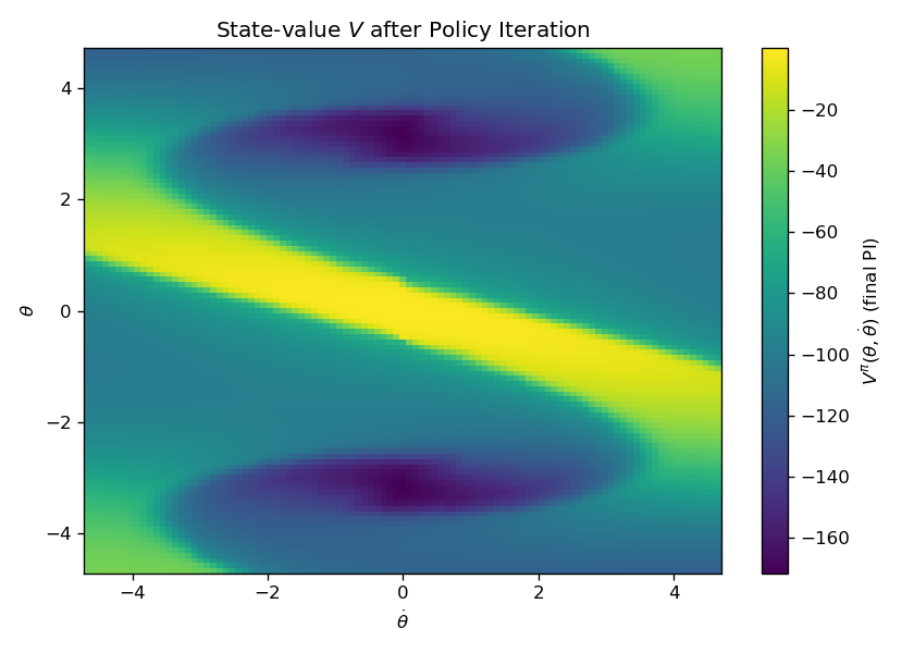
Figure 1.5: Optimal Value Function after Policy Iteration

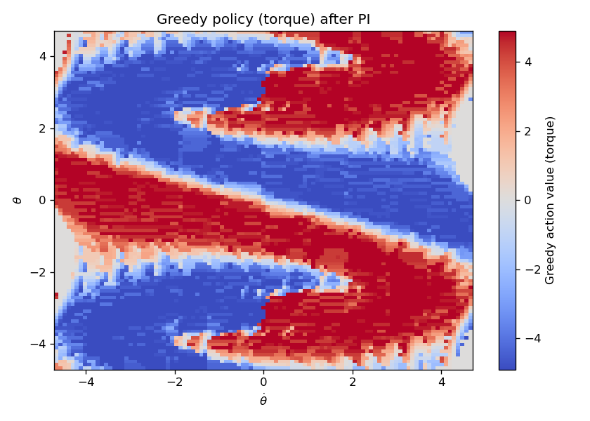
Figure 1.6: Optimal Policy after Policy Iteration

We can apply the optimal policy to the pendulum with an initial state of \((-\pi, 0)\) (i.e., the bottomright position). Fig. 1.7 plots the rollout trajectory of \(\theta, \dot{\theta}, u\). We can see that the optimal policy is capable of performing “bang-bang” control to accumulate energy before swinging up.

Fig. 1.8 overlays the trajectory on top of the optimal value function.

You can play with the code here.

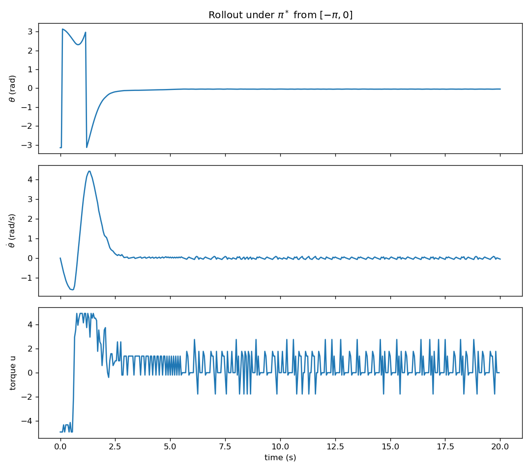
Figure 1.7: Optimal Trajectory of Pendulum Swing-Up

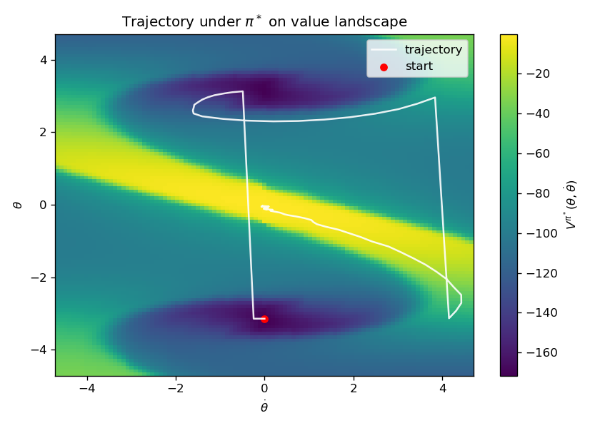
Figure 1.8: Optimal Trajectory of Pendulum Swing-Up Overlayed with Optimal Value Function

1.2.6 Value Iteration

Policy iteration—as the name suggests—iterates on policies: it alternates between (1) policy evaluation (computing \(V^{\pi}\) for the current policy \(\pi\)) and (2) policy improvement (making \(\pi\) greedy w.r.t. \(V^{\pi}\)).

An alternative, often very effective, method is value iteration. Unlike policy iteration, value iteration does not explicitly maintain a policy during its updates; it iterates directly on the value function toward the fixed point of the Bellman optimality* operator. Once the value function has (approximately) converged, the optimal policy is obtained by a single greedy extraction step. Note that intermediate value iterates need not correspond to the value of any actual policy.

The value iteration (VI) algorithm works as follows:

Initialization. Choose any \(V_0:\mathcal{S}\to\mathbb{R}\) (e.g., \(V_0 \equiv 0\)).
Iteration. For \(k=0,1,2,\dots\), \[ V_{k+1}(s) \;\leftarrow\; \max_{a\in\mathcal{A}} \Big[\, R(s,a) \;+\; \gamma \sum_{s'\in\mathcal{S}} P(s'\mid s,a)\; V_k(s') \,\Big], \quad \forall s\in\mathcal{S}. \] Stopping rule. Stop when \(\lVert V_{k+1}-V_k\rVert_\infty \le \varepsilon\) (or any chosen tolerance).

Policy extraction (greedy): \[ \pi_{k+1}(s) \in \arg\max_{a\in\mathcal{A}} \Big[\, R(s,a) \;+\; \gamma \sum_{s'} P(s'\mid s,a)\; V_{k+1}(s') \,\Big]. \]

The following theorem states the convergence of value iteration.

Theorem 1.4 (Convergence of Value Iteration) Let \(T^\star\) be the Bellman optimality operator, \[ (T^\star V)(s) := \max_{a}\Big[ R(s,a) + \gamma \sum_{s'} P(s'\mid s,a)\, V(s') \Big]. \] For \(\gamma\in[0,1)\) and finite \(\mathcal{S},\mathcal{A}\), \(T^\star\) is a \(\gamma\)-contraction in the sup-norm. Hence, for any \(V_0\), \[ V_k \;=\; (T^\star )^k V_0 \;\xrightarrow[k\to\infty]{}\; V^*, \] the unique fixed point of \(T^\star\). Moreover, the greedy policy \(\pi_k\) extracted from \(V_k\) converges to an optimal policy \(\pi^\star\).

In addition, after \(k\) iterations, we have \[ \lVert V_k - V^* \rVert_\infty \;\le\; \gamma^k \, \lVert V_0 - V^* \rVert_\infty. \]

Finally, we apply value iteration to the inverted pendulum problem.

Example 1.5 (Value Iteration for Inverted Pendulum) The following code performs value iteration for the inverted pendulum problem.

import numpy as np
import matplotlib.pyplot as plt

# ----- Physical & MDP parameters -----
g, l, m, c = 9.81, 1.0, 1.0, 0.1
dt = 0.05
gamma = 0.97
eps = 1e-8

# Grids
N_theta = 101
N_thetadot = 101
N_u = 51

theta_grid = np.linspace(-1.5*np.pi, 1.5*np.pi, N_theta)
thetadot_grid = np.linspace(-1.5*np.pi, 1.5*np.pi, N_thetadot)
u_max = 0.5 * m * g * l
u_grid = np.linspace(-u_max, u_max, N_u)

# Helpers to index/unwrap
def wrap_angle(x):
    return np.arctan2(np.sin(x), np.cos(x))

def state_index(i, j):
    return i * N_thetadot + j

def index_to_state(idx):
    i = idx // N_thetadot
    j = idx % N_thetadot
    return theta_grid[i], thetadot_grid[j]

S = N_theta * N_thetadot
A = N_u

# ----- Dynamics step (continuous -> one Euler step) -----
def step_euler(theta, thetadot, u):
    theta_next = wrap_angle(theta + dt * thetadot)
    thetadot_next = thetadot + dt * ((g/l) * np.sin(theta) + (1/(m*l*l))*u - c*thetadot)
    # clip angular velocity to grid range (bounded MDP)
    thetadot_next = np.clip(thetadot_next, thetadot_grid[0], thetadot_grid[-1])
    return theta_next, thetadot_next

# ----- Find 3 nearest grid states and probability weights (inverse-distance) -----
grid_pts = np.stack(np.meshgrid(theta_grid, thetadot_grid, indexing='ij'), axis=-1).reshape(-1, 2)

def nearest3_probs(theta_next, thetadot_next):
    x = np.array([theta_next, thetadot_next])
    dists = np.linalg.norm(grid_pts - x[None, :], axis=1)
    nn_idx = np.argpartition(dists, 3)[:3]      # three smallest (unordered)
    nn_idx = nn_idx[np.argsort(dists[nn_idx])]  # sort those 3 by distance
    d = dists[nn_idx]
    w = 1.0 / (d + eps)
    p = w / w.sum()
    return nn_idx.astype(int), p

# ----- Reward -----
def reward(theta, thetadot, u):
    return -(theta**2 + 0.1*thetadot**2 + 0.01*u**2)

# ----- Build tabular MDP: R[s,a] and sparse P[s,a,3] -----
R = np.zeros((S, A))
NS_idx = np.zeros((S, A, 3), dtype=int)   # next-state indices (3 nearest)
NS_prob = np.zeros((S, A, 3))             # their probabilities

for i, th in enumerate(theta_grid):
    for j, thd in enumerate(thetadot_grid):
        s = state_index(i, j)
        for a, u in enumerate(u_grid):
            R[s, a] = reward(th, thd, u)
            th_n, thd_n = step_euler(th, thd, u)
            nn_idx, p = nearest3_probs(th_n, thd_n)
            NS_idx[s, a, :] = nn_idx
            NS_prob[s, a, :] = p

# =======================
#       VALUE ITERATION
# =======================

# Bellman optimality update:
# V_{k+1}(s) = max_a [ R(s,a) + gamma * sum_j P(s,a,j) * V_k(ns_j) ]
V = np.zeros(S)
tol = 1e-6
max_vi_iters = 1000

for k in range(max_vi_iters):
    # Expected next V for every (s,a), given current V_k
    EV_next = (NS_prob * V[NS_idx]).sum(axis=2)   # shape (S, A)
    Q = R + gamma * EV_next                       # shape (S, A)
    V_new = np.max(Q, axis=1)                     # greedy backup over actions

    delta = np.max(np.abs(V_new - V))
    # Optional: a stopping rule aligned with policy loss bound could scale tol
    # e.g., stop when delta <= tol * (1 - gamma) / (2 * gamma)
    if delta < tol:
        V = V_new
        print(f"Value Iteration converged in {k+1} iterations (sup-norm change {delta:.2e}).")
        break
    V = V_new
else:
    print(f"Reached max_vi_iters={max_vi_iters} (last sup-norm change {delta:.2e}).")

# Greedy policy extraction from the final V
EV_next = (NS_prob * V[NS_idx]).sum(axis=2)   # recompute with final V
Q = R + gamma * EV_next
pi = np.argmax(Q, axis=1)                     # deterministic greedy policy (indices)

# ----- Visualization: Value function -----
V_grid = V.reshape(N_theta, N_thetadot)

fig, ax = plt.subplots(figsize=(7,5), dpi=120)
im = ax.imshow(
    V_grid,
    origin="lower",
    extent=[thetadot_grid.min(), thetadot_grid.max(),
            theta_grid.min(), theta_grid.max()],
    aspect="auto",
    cmap="viridis"
)
cbar = fig.colorbar(im, ax=ax)
cbar.set_label(r"$V^*(\theta,\dot{\theta})$ (Value Iteration)")

ax.set_xlabel(r"$\dot{\theta}$")
ax.set_ylabel(r"$\theta$")
ax.set_title(r"State-value $V$ after Value Iteration")

plt.tight_layout()
plt.show()

# ----- Visualization: Greedy torque field -----
pi_grid = pi.reshape(N_theta, N_thetadot)   # action indices
action_values = u_grid[pi_grid]             # map indices -> torques

plt.figure(figsize=(7,5), dpi=120)
im = plt.imshow(
    action_values,
    origin="lower",
    extent=[thetadot_grid.min(), thetadot_grid.max(),
            theta_grid.min(), theta_grid.max()],
    aspect="auto",
    cmap="coolwarm"   # good for ± torque
)
cbar = plt.colorbar(im)
cbar.set_label("Greedy action value (torque)")

plt.xlabel(r"$\dot{\theta}$")
plt.ylabel(r"$\theta$")
plt.title("Greedy policy (torque) extracted from Value Iteration")
plt.tight_layout()
plt.show()

Try it for yourself here!

You should obtain the same results as policy iteration.