Chapter 4 Model-based Planning and Optimization
In Chapter 1, we studied tabular MDPs with known dynamics where both the state and action spaces are finite, and we saw how dynamic-programming methods—Policy Iteration (PI) and Value Iteration (VI)—recover optimal policies.
Chapters 2 and 3 generalized these ideas to unknown dynamics and continuous spaces by introducing function approximation for value functions and policies. Those methods are model-free: they assume no access to the transition model and rely solely on data collected from interaction.
This chapter turns to the complementary regime: known dynamics with continuous state and action spaces. Our goal is to develop model-based planning and optimization methods that exploit the known dynamics to compute high-quality decisions efficiently.
We proceed in three steps:
Linear-quadratic systems. For linear dynamics and quadratic stage/terminal rewards (or costs), dynamic programming yields a linear optimal policy that can be computed efficiently via Riccati recursions. This setting serves as a tractable, illuminating baseline and a recurring building block in more general algorithms.
Trajectory optimization (TO) for nonlinear systems. When dynamics are nonlinear, we focus on planning an optimal state–action trajectory from a given initial condition, maximizing the cumulative reward (or minimizing cumulative cost) subject to dynamics and constraints. Unlike RL, which seeks an optimal feedback policy valid for all states, TO computes an open-loop plan (often with a time-varying local feedback around a nominal trajectory). Although less ambitious, TO naturally accommodates state/control constraints—common in motion planning under safety, actuation, and environmental limits—and is widely used in robotics and control.
Model predictive control (MPC). MPC converts open-loop plans into a feedback controller by repeatedly solving a short-horizon TO problem at each time step, applying only the first action, and receding the horizon. This receding-horizon strategy brings robustness to disturbances and model mismatch while retaining the constraint-handling benefits of TO.
We adopt the standard discrete-time dynamical system notation \[\begin{equation} x_{t+1} = f_t(x_t, u_t, w_t), \tag{4.1} \end{equation}\] where \(x_t \in \mathbb{R}^n\) is the state, \(u_t \in \mathbb{R}^m\) is the control/action, \(w_t \in \mathbb{R}^d\) is a (possibly stochastic) disturbance, and \(f_t\) is a known transition function, potentially nonlinear or nonsmooth. The goal is to find a policy that maximizes a sum of stage rewards \(r(x_t,u_t)\) and optional terminal reward \(r_T(x_T)\). We will often use the cost-minimization form \(c = -r\). State and action constraints are written as \[ x_t \in \mathcal{X}, \qquad u_t \in \mathcal{U}. \]
4.1 Linear Quadratic Regulator
In this section, we focus on the case when \(f_t\) is a linear function, and the rewards/costs are quadratic in \(x\) and \(u\). This family of problems is known as linear quadratic regulator (LQR).
4.1.1 Finite-Horizon LQR
Consider a linear discrete-time dynamical system \[\begin{equation} x_{k+1} = A_k x_k + B_k u_k + w_k, \quad k=0,1,\dots,N-1, \tag{4.2} \end{equation}\] where \(x_k \in \mathbb{R}^n\) the state, \(u_k \in \mathbb{R}^m\) the control, \(w_k \in \mathbb{R}^n\) the independent, zero-mean disturbance with given probability distribution that does not depend on \(x_k,u_k\), and \(A_k \in \mathbb{R}^{n \times n}, B_k \in \mathbb{R}^{n \times m}\) are known matrices determining the transition dynamics.
We want to solve the following optimal control problem \[\begin{equation} \min_{\mu_0,\dots,\mu_{N-1}} \mathbb{E} \left\{ x_N^\top Q_N x_N + \sum_{k=0}^{N-1} \left( x_k^\top Q_k x_k + u_k^\top R_k u_k \right) \right\}, \tag{4.3} \end{equation}\] where \(\mu_0,\dots,\mu_{N-1}\) are feedback policies/controllers that map states to actions and the expectation is taken over the randomness in \(w_0,\dots,w_{N-1}\). In (4.3), \(\{Q_k \}_{k=0}^N\) are positive semidefinite matrices, and \(\{ R_k \}_{k=0}^{N-1}\) are positive definite matrices. The formulation (4.3) is known as the linear quadratic regulator (LQR) problem because the dynamics is linear, the cost is quadratic, and the formulation can be considered to “regulate” the system around the origin \(x=0\).
The Bellman Optimality condition introduced in Theorem 1.1 still holds for continuous state and action spaces. Therefore, we will try to follow the dynamic programming (DP) algorithm in Section 1.1.4 to solve for the optimal policy.
The DP algorithm computes the optimal cost-to-go backwards in time. The terminal cost is \[ J_N(x_N) = x_N^\top Q_N x_N \] by definition.
The optimal cost-to-go at time \(N-1\) is equal to \[\begin{equation} \begin{split} J_{N-1}(x_{N-1}) = \min_{u_{N-1}} \mathbb{E}_{w_{N-1}} \{ x_{N-1}^\top Q_{N-1} x_{N-1} + u_{N-1}^\top R_{N-1} u_{N-1} + \\ \Vert \underbrace{A_{N-1} x_{N-1} + B_{N-1} u_{N-1} + w_{N-1} }_{x_N} \Vert^2_{Q_N} \} \end{split} \tag{4.4} \end{equation}\] where \(\Vert v \Vert_Q^2 = v^\top Q v\) for \(Q \succeq 0\). Now observe that the objective in (4.4) is \[\begin{equation} \begin{split} x_{N-1}^\top Q_{N-1} x_{N-1} + u_{N-1}^\top R_{N-1} u_{N-1} + \Vert A_{N-1} x_{N-1} + B_{N-1} u_{N-1} \Vert_{Q_N}^2 + \\ \mathbb{E}_{w_{N-1}} \left[ 2(A_{N-1} x_{N-1} + B_{N-1} u_{N-1} )^\top Q_{N-1} w_{N-1} \right] + \\ \mathbb{E}_{w_{N-1}} \left[ w_{N-1}^\top Q_N w_{N-1} \right] \end{split} \end{equation}\] where the second line is zero due to \(\mathbb{E}[w_{N-1}] = 0\) and the third line is a constant with respect to \(u_{N-1}\). Consequently, the optimal control \(u_{N-1}^\star\) can be computed by setting the derivative of the objective with respect to \(u_{N-1}\) equal to zero \[\begin{equation} u_{N-1}^\star = - \left[ \left( R_{N-1} + B_{N-1}^\top Q_N B_{N-1} \right)^{-1} B_{N-1}^\top Q_N A_{N-1} \right] x_{N-1}. \tag{4.5} \end{equation}\] Plugging the optimal controller \(u^\star_{N-1}\) back to the objective of (4.4) leads to \[\begin{equation} J_{N-1}(x_{N-1}) = x_{N-1}^\top S_{N-1} x_{N-1} + \mathbb{E} \left[ w_{N-1}^\top Q_N w_{N-1} \right], \tag{4.6} \end{equation}\] with \[ S_{N-1} = Q_{N-1} + A_{N-1}^\top \left[ Q_N - Q_N B_{N-1} \left( R_{N-1} + B_{N-1}^\top Q_N B_{N-1} \right)^{-1} B_{N-1}^\top Q_N \right] A_{N-1}. \] We note that \(S_{N-1}\) is positive semidefinite (this is an exercise for you to convince yourself).
Now we realize that something surprising and nice has happened.
The optimal controller \(u^{\star}_{N-1}\) in (4.5) is a linear feedback policy of the state \(x_{N-1}\), and
The optimal cost-to-go \(J_{N-1}(x_{N-1})\) in (4.6) is quadratic in \(x_{N-1}\), just the same as \(J_{N}(x_N)\).
This implies that, if we continue to compute the optimal cost-to-go at time \(N-2\), we will again compute a linear optimal controller and a quadratic optimal cost-to-go. This is the rare nice property for the LQR problem, that is,
The (representation) complexity of the optimal controller and cost-to-go does not grow as we run the DP recursion backwards in time.
We summarize the solution for the LQR problem (4.3) as follows.
Proposition 4.1 (Solution of Discrete-Time Finite-Horizon LQR) The optimal controller for the LQR problem (4.3) is a linear state-feedback policy \[\begin{equation} \mu_k^\star(x_k) = - K_k x_k, \quad k=0,\dots,N-1. \tag{4.7} \end{equation}\] The gain matrix \(K_k\) can be computed as \[ K_k = \left( R_k + B_k^\top S_{k+1} B_k \right)^{-1} B_k^\top S_{k+1} A_k, \] where the matrix \(S_k\) satisfies the following backwards recursion \[\begin{equation} \hspace{-6mm} \begin{split} S_N &= Q_N \\ S_k &= Q_k + A_k^\top \left[ S_{k+1} - S_{k+1}B_k \left( R_k + B_k^\top S_{k+1} B_k \right)^{-1} B_k^\top S_{k+1} \right] A_k, k=N-1,\dots,0. \end{split} \tag{4.8} \end{equation}\] The optimal cost-to-go is given by \[ J_0(x_0) = x_0^\top S_0 x_0 + \sum_{k=0}^{N-1} \mathbb{E} \left[ w_k^\top S_{k+1} w_k\right]. \] The recursion (4.8) is called the discrete-time Riccati equation.
Proposition 4.1 states that, to evaluate the optimal policy (4.7), one can first run the backwards Riccati equation (4.8) to compute all the positive definite matrices \(S_k\), and then compute the gain matrices \(K_k\). For systems of reasonable dimensions, evalutating the matrix inversion in (4.8) should be fairly efficient.
4.1.2 Infinite-Horizon LQR
We now switch to the infinite-horizon LQR problem \[\begin{align} \min_{\mu} & \quad \sum_{k=0}^{\infty} \left( x_k^\top Q x_k + u_k^\top R u_k \right) \tag{4.9} \\ \text{subject to} & \quad x_{k+1} = A x_k + B u_k, \quad k=0,\dots,\infty, \tag{4.10} \end{align}\] where \(Q \succeq 0\), \(R \succ 0\), \(A,B\) are constant matrices, and we seek a stationary policy \(\mu\) that maps states to actions. Note that here we remove the disturbance \(w_k\) because in general adding \(w_k\) will make the objective function unbounded. To handle \(w_k\), we will have to either add a discount factor \(\gamma\), or switch to an average cost objective function.
For infinite-horizon problems, the Bellman Optimality condition changes from a recursion to an equation. Specifically, according to Theorem 1.2 and equation (1.28), the optimal value function should satisfy the following Bellman optimality equation, restated for the case of cost minimization instead of reward maximization: \[\begin{equation} J^\star (x) = \min_{u} \left[ c(x,u) + \sum_{x'} P(x' \mid x, u) J^\star (x') \right], \quad \forall x, \tag{4.11} \end{equation}\] where \(c(x,u)\) is the cost function.
Guess A Solution. Based on our derivation in the finite-horizon case, we might as well guess that the optimal value function is a quadratic function: \[ J(x) = x^\top S x, \quad \forall x, \] for some positive definite matrix \(S\). Then, our guessed solution must satisfy the Bellman optimality stated in (4.11): \[\begin{equation} x^\top S x = J(x) = \min_{u} \left\{ x^\top Q x + u^\top R u + \Vert \underbrace{A x + B u}_{x'} \Vert_S^2 \right\}. \tag{4.12} \end{equation}\] The minimization over \(u\) in (4.12) can again be solved in closed-form by setting the gradient of the objective with respect to \(u\) to be zero \[\begin{equation} u^\star = - \underbrace{\left[ \left( R + B^\top S B \right)^{-1} B^\top S A \right]}_{K} x. \tag{4.13} \end{equation}\] Plugging the optimal \(u^\star\) back into (4.12), we see that the matrix \(S\) has to satisfy the following equation \[\begin{equation} S = Q + A^\top \left[ S - SB \left( R + B^\top S B \right)^{-1} B^\top S \right] A. \tag{4.14} \end{equation}\] Equation (4.14) is known as the discrete algebraic Riccati equation (DARE).
So the question boils down to if the DARE has a solution \(S\) that is positive definite?
Proposition 4.2 (Solution of Discrete-Time Infinite-Horizon LQR) Consider a linear system \[ x_{k+1} = A x_k + B u_k, \] with \((A,B)\) controllable (see Section 4.1.3). Let \(Q \succeq 0\) in (4.9) be such that \(Q\) can be written as \(Q = C^\top C\) with \((A,C)\) observable.
Then the optimal controller for the infinite-horizon LQR problem (4.9) is a stationary linear policy \[ \mu^\star (x) = - K x, \] with \[ K = \left( R + B^\top S B \right)^{-1} B^\top S A. \] The matrix \(S\) is the unique positive definite matrix that satisfies the discrete algebraic Riccati equation \[\begin{equation} S = Q + A^\top \left[ S - SB \left( R + B^\top S B \right)^{-1} B^\top S \right] A. \tag{4.15} \end{equation}\]
Moreover, the closed-loop system \[ x_{k+1} = A x_k + B (-K x_k) = (A - BK) x_k \] is stable, i.e., the eigenvalues of the matrix \(A - BK\) are strictly within the unit circle (see Appendix B.1.2).
Remark. The assumptions of \((A,B)\) being controllable and \((A,C)\) being observable can be relaxted to \((A,B)\) being stabilizable and \((A,C)\) being detectable (for definitions of stabilizability and detectability, see Appendix B).
We have not discussed how to solve the algebraic Riccati equation (4.15). It is clear that (4.15) is not a linear system of equations in \(S\). In fact, the numerical algorithms for solving the algebraic Riccati equation can be highly nontrivial, for example see (Arnold and Laub 1984). Fortunately, such algorithms are often readily available, and as practitioners we do not need to worry about solving the algebraic Riccati equation by ourselves. For example, the Matlab dlqr and the Python scipy.linalg.solve_discrete_are function computes the \(K\) and \(S\) matrices from \(A,B,Q,R\).
Let us now apply the infinite-horizon LQR solution to stabilizing a simple pendulum.
Example 4.1 (Pendulum Stabilization by LQR) Consider the simple pendulum in Fig. 4.1 with dynamics \[\begin{equation} x = \begin{bmatrix} \theta \\ \dot{\theta} \end{bmatrix}, \quad \dot{x} = f(x,u) = \begin{bmatrix} \dot{\theta} \\ -\frac{1}{ml^2}(b \dot{\theta} + mgl \sin \theta) + \frac{1}{ml^2} u \end{bmatrix} \tag{4.16} \end{equation}\] where \(m\) is the mass of the pendulum, \(l\) is the length of the pole, \(g\) is the gravitational constant, \(b\) is the damping ratio, and \(u\) is the torque applied to the pendulum.
We are interested in applying the LQR controller to balance the pendulum in the upright position \(x_d = [\pi,0]^\top\) with a zero velocity.
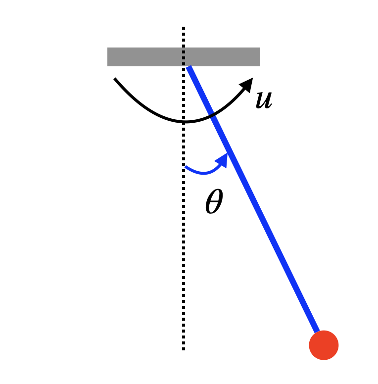
Figure 4.1: A Simple Pendulum.
Let us first shift the dynamics so that “\(0\)” is the upright position. This can be done by defining a new variable \(z = x - x_d = [\theta - \pi, \dot{\theta}]^\top\), which leads to \[\begin{equation} \dot{z} = \dot{x} = f(x,u) = f(z + x_d,u) = \begin{bmatrix} z_2 \\ \frac{1}{ml^2} \left( u - b z_2 + mgl \sin z_1 \right) \end{bmatrix} = f'(z,u). \tag{4.17} \end{equation}\] We then linearize the nonlinear dynamics \(\dot{z} = f'(z,u)\) at the point \(z^\star = 0, u^\star = 0\): \[\begin{align} \dot{z} & \approx f'(z^\star,u^\star) + \left( \frac{\partial f'}{\partial z} \right)_{z^\star,u^\star} (z - z^\star) + \left( \frac{\partial f'}{\partial u} \right)_{z^\star,u^\star} (u - u^\star) \\ & = \begin{bmatrix} 0 & 1 \\ \frac{g}{l} \cos z_1 & - \frac{b}{ml^2} \end{bmatrix}_{z^\star, u^\star} z + \begin{bmatrix} 0 \\ \frac{1}{ml^2} \end{bmatrix} u \\ & = \underbrace{\begin{bmatrix} 0 & 1 \\ \frac{g}{l} & - \frac{b}{ml^2} \end{bmatrix}}_{A_c} z + \underbrace{\begin{bmatrix} 0 \\ \frac{1}{ml^2} \end{bmatrix}}_{B_c} u. \end{align}\] Finally, we convert the continuous-time dynamics to discrete time with a fixed discretization \(h\) \[ z_{k+1} = \dot{z}_k \cdot h + z_k = \underbrace{(h \cdot A_c + I )}_{A} z_k + \underbrace{(h \cdot B_c)}_{B} u_k. \]
We are now ready to implement the LQR controller. In the formulation (4.9), we choose \(Q = I\), \(R = I\), and compute the gain matrix \(K\) by solving the DARE.
Fig. 4.2 shows the simulation result for \(m=1,l=1,b=0.1\), \(g = 9.8\), and \(h = 0.01\), with an initial condition \(z^0 = [0.1,0.1]^\top\). We can see that the LQR controller successfully stabilizes the pendulum at \(z^\star\), the upright position.
You can play with the Python code here.
Alternatively, the Matlab code can be found here.
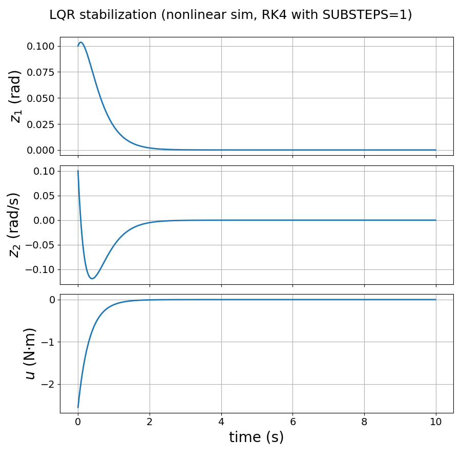
Figure 4.2: LQR stabilization of a simple pendulum.
4.1.3 Linear System Basics
Consider the discrete-time linear time-invariant (LTI) system \[ x_{k+1}=Ax_k+Bu_k,\qquad y_k=Cx_k+Du_k, \] with \(x_k\in\mathbb{R}^n,\;u_k\in\mathbb{R}^m,\;y_k\in\mathbb{R}^p\).
We provide a very brief review of linear system theory to understand Proposition 4.2. More details can be found in Appendix B.
Stability. The autonomous system \(x_{k+1}=Ax_k\) is (asymptotically) stable if for every \(x_0\) we have \(x_k\to 0\) as \(k\to\infty\).
Equivalent characterizations.
\(A\) is Schur: all eigenvalues satisfy \(|\lambda_i(A)|<1\).
Lyapunov: \(\exists P\succ 0\) s.t. \(A^\top P A - P \prec 0\).
Controllability (reachability). The pair \((A,B)\) is controllable if for any \(x_0,x_f\) there exists a finite input sequence \(\{u_0,\dots,u_{N-1}\}\) that drives the state from \(x_0\) to \(x_N=x_f\).
Kalman controllability matrix. \[ \mathcal C \;=\; [\,B\; AB\; A^2B\;\cdots\; A^{n-1}B\,],\quad \text{\((A,B)\) controllable} \iff \operatorname{rank}(\mathcal C)=n. \]
Popov-Belevitch-Hautus (PBH) test. \[ \text{\((A,B)\) controllable} \iff \operatorname{rank}\!\begin{bmatrix}\lambda I - A & B\end{bmatrix} = n \ \text{for all}\ \lambda\in\mathbb{C}. \] It suffices to check \(\lambda\) equal to the eigenvalues of \(A\).
Observability. The pair \((A,C)\) is observable if the initial state \(x_0\) can be uniquely determined from a finite sequence of outputs (and known inputs), e.g., from \(\{y_0,\dots,y_{n-1}\}\).
Observability matrix. \[ \mathcal O \;=\; \begin{bmatrix} C \\ CA \\ \vdots \\ CA^{n-1}\end{bmatrix},\quad \text{\((A,C)\) observable} \iff \operatorname{rank}(\mathcal O)=n. \]
PBH test. \[ \text{\((A,C)\) observable} \iff \operatorname{rank}\!\begin{bmatrix}\lambda I - A^\top & C^\top\end{bmatrix} = n \ \text{for all}\ \lambda\in\mathbb{C}. \] Dual to controllability: \((A,C)\) observable \(\Leftrightarrow\) \((A^\top,C^\top)\) controllable.
4.2 LQR Trajectory Tracking
Classical LQR delivers an optimal linear state-feedback when dynamics are linear and the objective is quadratic. In many planning problems, however, we do not seek a single stationary feedback for all states but rather a local stabilizer around a given (possibly time-varying) trajectory—for instance, a motion plan from a trajectory optimizer or MPC’s rolling nominal (see Section 4.3). LQR Tracking (also called time-varying LQR, TVLQR) provides exactly this: a time-varying linear feedback that stabilizes the system near a nominal state–control sequence and rejects small disturbances.
Problem Setup. Let the nominal (i.e., ignoring the disturbance) discrete-time system be \[ x_{t+1} \;=\; f_t(x_t,u_t), \qquad t=0,\dots,N-1, \] and suppose we have a nominal trajectory \(\{(\bar x_t,\bar u_t)\}_{t=0}^{N-1}\) satisfying \[ \bar x_{t+1} \;=\; f_t(\bar x_t,\bar u_t). \]
Our goal is to design a controller that can stabilize the system with disturbance, i.e., \(x_{t+1} = f_t(x_t, u_t, w_t)\), around the nominal trajectory.
Towards this, we define deviations from the nominal trajectory as \[ \delta x_t := x_t-\bar x_t, \qquad \delta u_t := u_t-\bar u_t. \]
If the true system is linear time-varying (or we linearize a nonlinear system along the nominal), we obtain the deviation dynamics \[ \delta x_{t+1} \;\approx\; A_t\,\delta x_t + B_t\,\delta u_t, \quad A_t := \left.\frac{\partial f_t}{\partial x}\right|_{(\bar x_t,\bar u_t)},\quad B_t := \left.\frac{\partial f_t}{\partial u}\right|_{(\bar x_t,\bar u_t)}. \tag{4.18} \]
We penalize deviations with a quadratic cost \[ J \;=\; \delta x_N^\top Q_N \delta x_N \;+\;\sum_{t=0}^{N-1} \Big(\delta x_t^\top Q_t \delta x_t \;+\; \delta u_t^\top R_t \delta u_t\Big), \quad Q_t\succeq 0,\; R_t\succ 0. \tag{4.19} \]
LQR Tracking Algorithm. The tracking controller takes the affine form \[ u_t \;=\; \bar u_t \;-\; K_t\,(x_t-\bar x_t), \] where \(\{K_t\}_{t=0}^{N-1}\) are time-varying gains computed by a backward Riccati recursion on the deviation system (4.18) with cost (4.19).
From Proposition 4.1, we know the gains can be computed as follows.
Initialize at terminal time: \[ S_N \;=\; Q_N. \] For \(t = N-1,\,N-2,\,\dots,\,0\): \[\begin{equation} \begin{split} K_t &= \Big(R_t + B_t^\top S_{t+1} B_t\Big)^{-1} B_t^\top S_{t+1} A_t, \\[2mm] S_t &= Q_t \;+\; A_t^\top \!\Big(S_{t+1} - S_{t+1} B_t \big(R_t + B_t^\top S_{t+1} B_t\big)^{-1} B_t^\top S_{t+1}\Big) A_t. \end{split} \tag{4.20} \end{equation}\]
Given the gains \(\{K_t\}\), apply at runtime: \[\begin{equation} u_t \;=\; \bar u_t - K_t\,(x_t-\bar x_t), \qquad t=0,\dots,N-1. \tag{4.21} \end{equation}\]
The following pseudocode summarizes the algorithm.
Algorithm: LQR Trajectory Tracking (TVLQR)
Inputs: nominal \(\{(\bar x_t,\bar u_t)\}_{t=0}^{N-1}\), weights \(\{Q_t,R_t\}\), terminal \(Q_N\).
- Linearize along the nominal to get \(A_t,B_t\) via (4.18).
- Backward pass: compute \(K_t\) and \(S_t\) via (4.20).
- Apply feedback: \(u_t=\bar u_t - K_t(x_t-\bar x_t)\) as in (4.21).
Output: time-varying gains \(\{K_t\}\) giving a local stabilizer around the trajectory.
We now apply TVLQR to a vehicle trajectory tracking problem.
Example 4.2 (LQR Trajectory Tracking for Unicyle) We (i) define the dynamics in continuous and discrete time, (ii) specify a circular nominal trajectory, (iii) linearize the nonlinear dynamics along the nominal, (iv) state the deviation-cost weights \(Q,R\) (and terminal \(Q_N\)), and (v) list the experiment setup (discretization and horizon length).
Unicycle Dynamics (Continuous and Discrete).
State and input.
\[
x=\begin{bmatrix}p_x\\ p_y\\ \theta\end{bmatrix}\in\mathbb{R}^3,
\qquad
u=\begin{bmatrix}v\\ \omega\end{bmatrix}\in\mathbb{R}^2,
\]
where \((p_x,p_y)\) is planar position, \(\theta\) is heading, \(v\) is forward speed, and \(\omega\) is yaw rate.
Continuous time: \[\begin{equation} \dot p_x = v\cos\theta,\qquad \dot p_y = v\sin\theta,\qquad \dot\theta = \omega. \tag{4.22} \end{equation}\]
Discrete time (forward Euler with step \(h>0\)): \[\begin{equation} x_{t+1} \;=\; f(x_t,u_t) := \begin{bmatrix} p_{x,t} + h\, v_t\cos\theta_t\\[2pt] p_{y,t} + h\, v_t\sin\theta_t\\[2pt] \theta_t + h\,\omega_t \end{bmatrix}. \tag{4.23} \end{equation}\]
Nominal Trajectory (Circular Motion). We track a circle of radius \(R=\dfrac{\bar v}{\bar\omega}\) using constant nominal inputs \[\begin{equation} \bar u_t \equiv \begin{bmatrix}\bar v\\ \bar\omega\end{bmatrix},\qquad t=0,\dots,N-1, \tag{4.24} \end{equation}\] and generate the nominal state recursively under the discrete dynamics (4.23): \[\begin{equation} \bar x_{t+1} \;=\; f(\bar x_t,\bar u_t),\qquad \bar x_0 = \begin{bmatrix}R\\ 0\\ \frac{\pi}{2}\end{bmatrix}. \tag{4.25} \end{equation}\]
We define deviations from the nominal: \[ \delta x_t := x_t-\bar x_t,\qquad \delta u_t := u_t-\bar u_t. \]
Linearization Along the Nominal. Linearize (4.23) at \((\bar x_t,\bar u_t)\) to obtain the deviation dynamics \[\begin{equation} \delta x_{t+1} \;\approx\; A_t\,\delta x_t + B_t\,\delta u_t, \tag{4.26} \end{equation}\] with Jacobians (using \(c_t:=\cos\bar\theta_t,\ s_t:=\sin\bar\theta_t\)) \[\begin{equation} A_t \;=\; \frac{\partial f}{\partial x}\Big|_{(\bar x_t,\bar u_t)} = \begin{bmatrix} 1 & 0 & -h\,\bar v\,s_t\\ 0 & 1 & \ \ h\,\bar v\,c_t\\ 0 & 0 & 1 \end{bmatrix}, \qquad B_t \;=\; \frac{\partial f}{\partial u}\Big|_{(\bar x_t,\bar u_t)} = \begin{bmatrix} h\,c_t & 0\\ h\,s_t & 0\\ 0 & h \end{bmatrix}. \tag{4.27} \end{equation}\]
Deviation Cost (Weights \(Q,R,Q_N\)). We penalize deviations with a quadratic stage/terminal cost \[ J \;=\; \delta x_N^\top Q_N\,\delta x_N \;+\;\sum_{t=0}^{N-1}\Big(\delta x_t^\top Q\,\delta x_t+\delta u_t^\top R\,\delta u_t\Big), \] using the weights: \[\begin{equation} Q=\mathrm{diag}(30,\;30,\;5),\qquad Q_N=\mathrm{diag}(60,\;60,\;8),\qquad R=\mathrm{diag}(0.2,\;0.2). \tag{4.28} \end{equation}\] These reflect a stronger emphasis on position tracking, a moderate penalty on heading error, and a mild penalty on control deviations from the nominal.
Experiment Setup.
- Discretization step: \(h = 0.02\ \mathrm{s}\).
- Horizon length: \(T_{\mathrm{final}} = 12\ \mathrm{s}\).
- Number of steps: \(N = T_{\mathrm{final}}/h = \mathbf{600}\).
- Nominal inputs: \(\bar v = 1.2\ \mathrm{m/s},\ \bar\omega = 0.4\ \mathrm{rad/s}\) (radius \(R=\bar v/\bar\omega\)).
- Initialization: the nominal starts at \(\bar x_0 = [\,R,\,0,\,\pi/2\,]^\top\); the actual system may start with a small offset (see code).
With \((A_t,B_t)\) from (4.27) and weights (4.28), the TVLQR backward Riccati recursion (Section 4.2) yields gains \(K_t\). We then apply the local feedback \[ u_t \;=\; \bar u_t - K_t\,(x_t-\bar x_t), \] to robustly track the circular nominal under small disturbances.
Disturbances. To test robustness, we inject additive process disturbances into the discrete dynamics: \[ x_{t+1} \;=\; f(x_t,u_t)\;+\; w_t,\qquad t=0,\dots,N-1, \] where \[ w_t \;=\; \underbrace{\eta_t}_{\text{i.i.d. Gaussian noise}} \;+\; \underbrace{g_t}_{\text{deterministic gust}}. \]
Small i.i.d. Gaussian process noise. We draw \(\eta_t \sim \mathcal N(0,W)\) independently at each step with \[ W \;=\; \mathrm{diag}\!\big(\sigma_x^2,\ \sigma_y^2,\ \sigma_\theta^2\big), \qquad \sigma_x = \sigma_y = 0.01\ \text{m},\quad \sigma_\theta = \mathrm{deg2rad}(0.2). \] This noise perturbs the post-update state components \((p_x,p_y,\theta)\).
Finite-duration “gust” impulse. In addition to \(\eta_t\), we apply a brief deterministic bias over a window \[ t \in [t_g,\ t_g+\Delta] \;=\; [\,4.0\,\mathrm{s},\ 4.8\,\mathrm{s}\,), \] implemented at the discrete indices \(\{t_g,\dots,t_g+\Delta\}\). During this window we set \[ g_t \;=\; \begin{bmatrix} \delta p_x \\[1mm] 0 \\[1mm] \delta \theta \end{bmatrix}, \qquad \delta p_x = 0.01\ \text{m per step},\quad \delta \theta = \mathrm{deg2rad}(1.8)\ \text{per step}, \] and \(g_t=\mathbf{0}\) otherwise. This models a short-lived lateral drift and a heading kick.
Results. Fig. 4.3 visualizes the nominal trajectory (the dotted circle) and the TVLQR-stabilized trajectory in blue. To clearly see the impact of closed-loop LQR tracking, we also plotted the open-loop trajectory, i.e., the system’s trajectory if no feedback is applied. We can observe that the TVLQR controller effectively rejects the disturbances and stabilizes the closed-loop trajectory along the nominal path.
Fig. 4.4 visualizes the state tracking error (position and heading error) as well as compares the closed-loop control with open-loop control.
You can play with the code here.
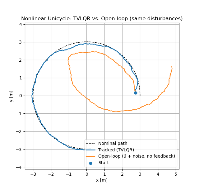
Figure 4.3: LQR Trajectory Tracking for Unicyle: comparison between nominal trajectory, open-loop trajectory, and closed-loop trajectory with feedback.
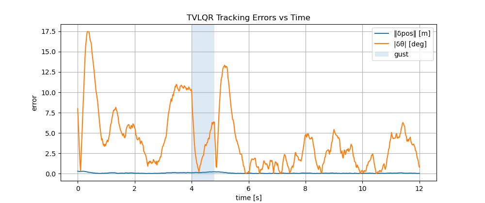
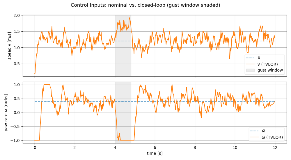
Figure 4.4: LQR Trajectory Tracking for Unicyle: state tracking error (top) and control signal (bottom).
4.3 Trajectory Optimization
In Section 4.2 we saw that TVLQR gives a powerful local stabilizer around a nominal state–control sequence \((\bar x_t,\bar u_t)\). This raises a natural question:
Where do nominal trajectories come from?
In many robotics tasks (maneuvering a car, landing a rocket, walking with a robot), we must compute a feasible, high-quality open-loop plan that respects the dynamics and constraints. Trajectory Optimization (TO) does exactly this: it searches over sequences \(\{x_t,u_t\}\) to minimize a cumulative cost while satisfying the system dynamics and constraints.
Moreover, if we can solve TO quickly (or approximately, but reliably), then by re-solving over a short horizon at each time step and applying only the first control, we obtain Model Predictive Control (MPC)—a feedback controller that blends optimization with robustness (see Section 4.4 later). Thus, TO is both a planner and the engine behind feedback via MPC.
General Nonlinear Trajectory Optimization Problem. We adopt the standard discrete-time nonlinear system \[ x_{t+1} = f_t(x_t,u_t),\qquad t=0,\dots,N-1, \] with state \(x_t\in\mathbb{R}^n\) and control \(u_t\in\mathbb{R}^m\). A generic finite-horizon TO problem is \[\begin{equation} \begin{split} \min_{\{x_t,u_t\}} \quad & \Phi(x_N) + \sum_{t=0}^{N-1} \ell_t(x_t,u_t) \\[2mm] \text{s.t.}\quad & x_{t+1} = f_t(x_t,u_t), \qquad t=0,\dots,N-1,\\ & x_0 = \hat x_0 \ \ \text{(given)},\\ & x_t \in \mathcal X_t,\quad u_t \in \mathcal U_t \quad \text{(bounds)},\\ & g_t(x_t,u_t) \le 0,\quad h_t(x_t,u_t)=0 \quad \text{(path/terminal constraints).} \end{split} \tag{4.29} \end{equation}\] Here \(\ell_t\) and \(\Phi\) encode performance (e.g., energy, time, tracking error), \(\mathcal X_t,\mathcal U_t\) capture box limits and safety sets, and \(g_t,h_t\) represent additional nonlinear constraints (obstacles, terminal goals, etc.).
Solving (4.29) directly is difficult in general. A widely used strategy is to iteratively approximate it by quadratic subproblems that can be solved efficiently. This leads to iLQR and its second-order cousin DDP (see Section 4.3.2).
4.3.1 Iterative LQR
High-level intuition. iLQR (iterative LQR) alternates between:
Local modeling: around a current nominal trajectory \(\{(\bar x_t,\bar u_t)\}\),
- linearize the dynamics,
- quadratically approximate the cost.
- linearize the dynamics,
LQR step: solve the resulting time-varying LQR subproblem to obtain a time-varying affine policy \[ \delta u_t = k_t + K_t\,\delta x_t,\quad \delta x_t:=x_t-\bar x_t,\ \delta u_t:=u_t-\bar u_t, \] which gives both a feedforward step \(k_t\) (to change the nominal control) and a feedback gain \(K_t\) (to stabilize the rollout).
Forward rollout + line search: apply \(u_t^{\text{new}}=\bar u_t+\alpha k_t + K_t(x_t^{\text{new}}-\bar x_t)\) to the true nonlinear dynamics, producing a new nominal trajectory \(\{(\bar x_t,\bar u_t)\}\). Here we choose \(\alpha\in(0,1]\) to reduce the cost and respect constraints.
Repeat until convergence (cost decrease and dynamics residuals are small).
iLQR can be viewed as a Gauss–Newton method on trajectories: it uses first-order dynamics and second-order cost, capturing the dominant curvature while remaining numerically robust and fast.
4.3.1.1 LQR Subproblem (one iLQR outer iteration)
Given a nominal trajectory \(\{(\bar x_t,\bar u_t)\}_{t=0}^{N-1}\) with \(\bar x_{t+1}=f_t(\bar x_t,\bar u_t)\), define deviations \[ \delta x_t := x_t-\bar x_t,\qquad \delta u_t := u_t-\bar u_t,\qquad \delta x_0\ \text{given.} \]
Linearized Dynamics. We linearize the dynamics along the nominal trajectory \[ \delta x_{t+1} \;\approx\; A_t\,\delta x_t + B_t\,\delta u_t,\quad A_t:=\left.\frac{\partial f_t}{\partial x}\right|_{(\bar x_t,\bar u_t)},\ \ B_t:=\left.\frac{\partial f_t}{\partial u}\right|_{(\bar x_t,\bar u_t)}. \tag{4.30} \]
Quadratic Cost Approximation. We perform a quadratic approximation of the objective function about \((\bar x_t,\bar u_t)\) \[ \begin{aligned} \ell_t(x_t,u_t) &\approx \ell_t + \ell_{x,t}^\top \delta x_t + \ell_{u,t}^\top \delta u_t + \frac{1}{2} \begin{bmatrix}\delta x_t\\ \delta u_t\end{bmatrix}^{\!\top} \!\begin{bmatrix}\ell_{xx,t} & \ell_{xu,t}\\ \ell_{ux,t} & \ell_{uu,t}\end{bmatrix} \!\begin{bmatrix}\delta x_t\\ \delta u_t\end{bmatrix},\\ \Phi(x_N) &\approx \Phi + \Phi_x^\top \delta x_N + \frac{1}{2}\,\delta x_N^\top \Phi_{xx}\,\delta x_N. \end{aligned} \tag{4.31} \]
The LQR Subproblem. With (4.30)–(4.31), the iLQR subproblem at this outer iteration is the finite-horizon linear–quadratic program in deviations: \[ \begin{aligned} \min_{\{\delta x_t,\delta u_t\}} \quad & \underbrace{\frac{1}{2}\,\delta x_N^\top \Phi_{xx}\,\delta x_N + \Phi_x^\top \delta x_N}_{\text{terminal}} \;+\; \\ & \sum_{t=0}^{N-1} \underbrace{\Big( \frac{1}{2} \begin{bmatrix}\delta x_t\\ \delta u_t\end{bmatrix}^{\!\top} \!\begin{bmatrix}\ell_{xx,t} & \ell_{xu,t}\\ \ell_{ux,t} & \ell_{uu,t}\end{bmatrix} \!\begin{bmatrix}\delta x_t\\ \delta u_t\end{bmatrix} + \ell_{x,t}^\top\delta x_t + \ell_{u,t}^\top\delta u_t \Big)}_{\text{stage}} \\[1mm] \text{s.t.}\quad & \delta x_{t+1} = A_t\,\delta x_t + B_t\,\delta u_t,\qquad t=0,\dots,N-1,\\ & \delta x_0\ \text{given.} \end{aligned} \tag{4.32} \]
Notes. The iLQR subproblem (4.32) is slightly different from the previous finite-horizon LQR formulation (4.3) in the sense that the objective function of (4.32) also contains linear terms in \(\delta x_t,\delta u_t\), and those linear terms come from the Taylor expansion of the original nonlinear objective fuctions. In this case, we will see in the following that the optimal policy is affine (feedforward \(k_t\) + feedback \(K_t\)).
4.3.1.2 Solving the Subproblem by Dynamic Programming
We posit a quadratic value approximator at each time: \[ V_{t}(\delta x_{t}) \;\approx\; V_{t} + V_{x,t}^\top \delta x_t + \frac{1}{2}\,\delta x_t^\top V_{xx,t}\,\delta x_t, \qquad V_{x,N}=\Phi_x,\; V_{xx,N}=\Phi_{xx}. \tag{4.33} \] Note that this quadratic value approximator also contains linear and constant terms because the objective function contains linear terms.
Define the local Q-function at stage \(t\) by substituting the linear dynamics into the next-step value (this is our familiar Q-value in RL): \[ Q_t(\delta x_t,\delta u_t) \;=\; \ell_t(x_t,u_t) + V_{t+1} \big(A_t\delta x_t + B_t\delta u_t\big), \] which, after collecting terms, yields the iLQR blocks \[ \begin{aligned} Q_{x,t}&=\ell_{x,t}+A_t^\top V_{x,t+1},\qquad Q_{u,t}=\ell_{u,t}+B_t^\top V_{x,t+1},\\ Q_{xx,t}&=\ell_{xx,t}+A_t^\top V_{xx,t+1}A_t,\quad Q_{ux,t}=\ell_{ux,t}+B_t^\top V_{xx,t+1}A_t,\\ Q_{uu,t}&=\ell_{uu,t}+B_t^\top V_{xx,t+1}B_t. \end{aligned} \tag{4.34} \] The iLQR blocks assemble into a big matrix such that \[ Q_t(\delta x_t,\delta u_t) \;=\; \frac{1}{2}\, \begin{bmatrix} 1 \\ \delta x_t \\ \delta u_t \end{bmatrix}^\top \begin{bmatrix} 2c_t & Q_{x,t}^\top & Q_{u,t}^\top\\[2pt] Q_{x,t} & Q_{xx,t} & Q_{xu,t}\\[2pt] Q_{u,t} & Q_{ux,t} & Q_{uu,t} \end{bmatrix} \begin{bmatrix} 1 \\ \delta x_t \\ \delta u_t \end{bmatrix}. \tag{4.35} \] where \(c_t\) collects all stage/terminal constants e.g., \(\ell_t+\!V_{t+1}\).
Solving the local Q (backward pass). Set the first-order condition w.r.t. \(\delta u\): \[ 0 \;=\; \partial_{\delta u} Q_t \;=\; Q_{u,t} + Q_{ux,t}\delta x + Q_{uu,t}\delta u. \] Solve for the affine control law \[ \delta u_t^\star \;=\; k_t + K_t\,\delta x,\qquad k_t = -Q_{uu,t}^{-1} Q_{u,t},\quad K_t = -Q_{uu,t}^{-1} Q_{ux,t}\!, \tag{4.36} \] which is exactly the LQR solution for the quadratic \(Q_t\).
Substitute \(\delta u_t^\star\) back into (4.35). The minimized Q becomes a quadratic in \(\delta x\) with coefficients given by \[ \begin{aligned} V_{x,t} &= Q_{x,t} + Q_{xu,t}k_t + K_t^\top Q_{uu,t}k_t + K_t^\top Q_{u,t},\\ V_{xx,t} &= Q_{xx,t} + Q_{xu,t}K_t + K_t^\top Q_{ux,t} + K_t^\top Q_{uu,t}K_t, \end{aligned} \tag{4.37} \] with terminal \[ V_{x,N} = \Phi_x, V_{xx,N} = \Phi_{xx}. \]
Forward Pass (apply the computed policy). Given \(\{k_t,K_t\}\), produce a candidate trajectory on the true nonlinear dynamics using a line search \(\alpha\in(0,1]\): \[ \begin{aligned} u_t^{\text{cand}} &= \bar u_t + \alpha k_t + K_t\big(x_t^{\text{cand}}-\bar x_t\big) ,\\ x_{t+1}^{\text{cand}} &= f_t\big(x_t^{\text{cand}},u_t^{\text{cand}}\big),\qquad x_0^{\text{cand}}=\hat x_0. \end{aligned} \tag{4.38} \] Choose \(\alpha\) (e.g., \(\{1,\frac{1}{2},\frac14,\dots\}\)) to reduce the true cost and respect constraints, then update the nominal: \[ (\bar x_t,\bar u_t)\ \leftarrow\ (x_t^{\text{cand}},u_t^{\text{cand}}). \]
The following pseudocode summarizes iLQR.
Algorithm: iLQR (Trajectory Generation)
Inputs: dynamics \(f_t\), initial state \(\hat x_0\), horizon \(N\), stage/terminal costs \(\ell_t,\Phi\), initial guess \(\{\bar u_t\}\).
- Initialize nominal rollout \(\{\bar x_t,\bar u_t\}\) from \(\hat x_0\).
- Linearize & quadratize at \(\{(\bar x_t,\bar u_t)\}\): build \(A_t,B_t\) and cost derivatives.
- Backward pass (TVLQR): compute \(\{k_t,K_t\}\) using (4.36) and update \(V_{x,t},V_{xx,t}\) via (4.37).
- Forward rollout: apply \(u_t^{\text{new}}=\bar u_t+\alpha k_t+K_t(x_t^{\text{new}}-\bar x_t)\) on the true dynamics, pick \(\alpha\) by line search.
- Convergence check: stop if the cost decrease and dynamics residuals fall below thresholds; otherwise, set the new nominal and repeat from Step 2.
The next example applies iLQR to trajectory generation for rocket landing.
Example 4.3 (iLQR for Rocket Landing) We model a planar (2D) rocket with state and control \[ x=\begin{bmatrix}p_x & p_y & v_x & v_y & \theta & \omega\end{bmatrix}^\top,\qquad u=\begin{bmatrix}T & \tau\end{bmatrix}^\top, \] where \((p_x,p_y)\) is position, \((v_x,v_y)\) is velocity, \(\theta\) is attitude (pitch) and \(\omega\) its angular rate. The thrust \(T\ge 0\) acts along the body axis (pointing out of the engine), and \(\tau\) is a planar torque about the center of mass. Continuous-time dynamics are \[ \begin{aligned} \dot p_x &= v_x, & \dot p_y &= v_y, \\ \dot v_x &= \frac{T}{m}\sin\theta, & \dot v_y &= \frac{T}{m}\cos\theta - g, \\ \dot\theta &= \omega, & \dot\omega &= \frac{\tau}{I_{zz}}. \end{aligned} \tag{4.39} \] In simulation we use RK4 with stepsize \(h\) to propagate the true dynamics (4.39). For iLQR’s local subproblems we form the continuous Jacobians \((A_c,B_c)=\big(\frac{\partial f}{\partial x},\frac{\partial f}{\partial u}\big)\) at the current nominal and use the standard first-order discrete map \[ A_t \;\approx\; I + h\,A_c(\bar x_t,\bar u_t),\qquad B_t \;\approx\; h\,B_c(\bar x_t,\bar u_t). \tag{4.40} \]
Soft-Landing Objective. The goal is a soft, upright landing at the origin: \[ x_{\mathrm{goal}} = \mathbf{0} \quad\Longleftrightarrow\quad p_x=p_y=0,\; v_x=v_y=0,\; \theta=0,\; \omega=0. \] We penalize deviations from this goal along the entire trajectory and especially at the terminal state to encourage low touchdown velocities and an upright attitude.
Cost Function. With horizon \(N\) and step \(h\), the discrete objective is \[ J \;=\; \frac{1}{2}\,(x_N-x_g)^\top Q_f (x_N-x_g) \;+\;\sum_{t=0}^{N-1}\Big[ \frac{1}{2}\,(x_t-x_g)^\top Q (x_t-x_g) \;+\; \frac{1}{2}\,u_t^\top R u_t \Big], \tag{4.41} \] where \(x_g=\mathbf{0}\). In the example: \[ \begin{aligned} Q&=\mathrm{diag}(1,\ 2,\ 0.5,\ 0.5,\ 2,\ 0.5),\\ Q_f&=\mathrm{diag}(200,\ 300,\ 50,\ 50,\ 300,\ 50),\\ R&=\mathrm{diag}(10^{-3},\ 10^{-3}). \end{aligned} \tag{4.42} \] These weights place strong emphasis on terminal altitude and attitude (\(p_y,\theta\)), moderate emphasis on velocities and lateral position, and a light regularization on the controls.
Experiment Setup.
Physical parameters. Gravity \(g=9.81\,\mathrm{m/s^2}\), mass \(m=1.0\,\mathrm{kg}\), planar inertia \(I_{zz}=0.2\,\mathrm{kg\,m^2}\).
Discretization. Stepsize \(h=0.05\,\mathrm{s}\); horizon \(T=6.0\,\mathrm{s}\); number of steps \(N=T/h=120\).
Initial state. \[ x_0=\big[\,5.0,\ 10.0,\ -0.5,\ -1.0,\ \mathrm{deg2rad}(10),\ 0\,\big]^\top, \] i.e., 10 m altitude, lateral offset, small descent and slight pitch.
Initial nominal controls. Constant hover thrust and zero torque: \[ \bar u_t = [\,m g,\ 0\,]^\top,\qquad t=0,\dots,N-1. \]
iLQR procedure. Each outer iteration:
- Linearize dynamics and quadratize the cost along the current nominal ((4.40), (4.41));
- Solve the time-varying LQR subproblem to get affine updates \(\delta u_t = k_t + K_t\,\delta x_t\);
- Forward rollout on the nonlinear RK4 dynamics with
\[
u_t^{\text{new}} = \bar u_t + \alpha\,k_t + K_t\big(x_t^{\text{new}}-\bar x_t\big),
\]
using a backtracking line search over \(\alpha\in\{1,\frac{1}{2},\frac14,\dots\}\) (note: \(\alpha\) scales only the feedforward \(k_t\), not the feedback \(K_t\));
- Update the nominal and repeat until cost reduction is small.
- Linearize dynamics and quadratize the cost along the current nominal ((4.40), (4.41));
Fig. 4.5 plots the initial, intermediate, and final trajectories, and render the rocket as oriented rectangles (boxes) using \((p_x,p_y,\theta)\) to visualize attitude along the descent. We can see iLQR successfully generated a soft landing trajectory.
You can play with the code here.
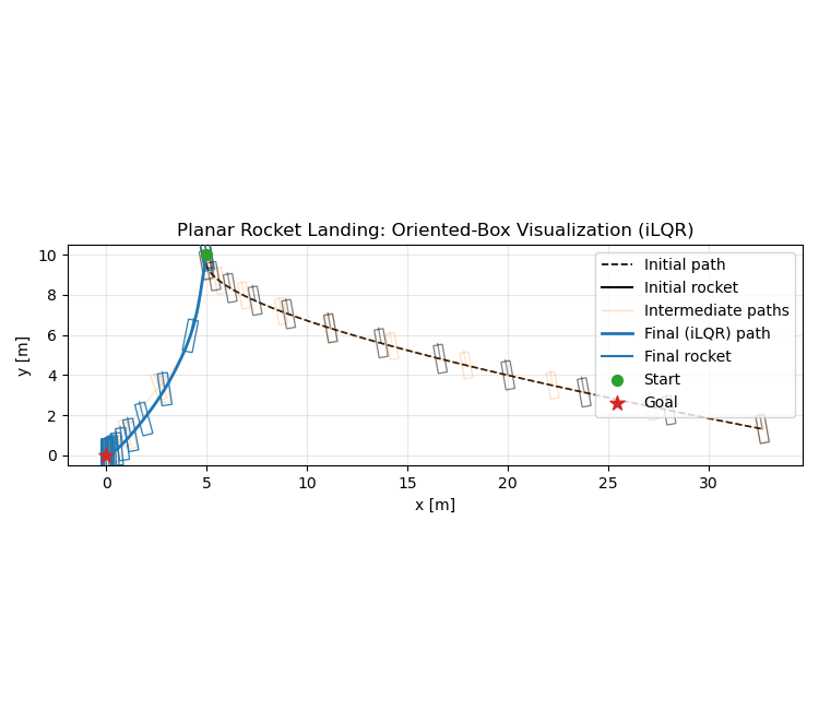
Figure 4.5: iLQR Trajectory Generation for Rocket Landing.
4.3.3 Quadratic Programming
Trajectory optimization (TO) with nonlinear dynamics and objectives is well served by iLQR/DDP: at each outer iteration, they linearize the dynamics and quadratize the objective, then solve a time-varying LQR subproblem. This works remarkably well for unconstrained or softly constrained problems.
However, many TO tasks are constrained—e.g., obstacle avoidance, actuator limits, keep-out zones, terminal envelopes. Hard constraints are awkward for iLQR/DDP (they typically enter via penalties or saturations), and feasibility can be fragile. For such cases, it is often more natural to frame TO as a nonlinear program (NLP)—an optimization problem with general nonlinear objective and constraints. This brings the full machinery of modern numerical optimization (see, e.g., (Nocedal and Wright 1999)).
As a first step, we study the convex special case where the linearization already yields linear dynamics, affine constraints, and a quadratic objective (these are typically known as “constrained LQR” problems). This leads to Quadratic Programming (QP), a cornerstone problem class with mature, efficient solvers. In the next section, we will lift these ideas to Sequential Quadratic Programming (SQP) to handle general constrained TO.
4.3.3.1 From Trajectory Optimization to Quadratic Programming
Start from the constrained TO template in (4.29). Suppose:
- Linear (time-varying) dynamics (from linearization or an intrinsically linear model): \[ x_{t+1} = A_t x_t + B_t u_t + a_t,\qquad t=0,\dots,N-1, \] with given \(x_0=\hat x_0\).
- Quadratic objective (from quadratization or an Linear-Quadratic tracking design): \[ \Phi(x_N) + \sum_{t=0}^{N-1} \ell_t(x_t,u_t) \;\equiv\; \frac{1}{2}\,x_N^\top Q_N x_N + q_N^\top x_N + \sum_{t=0}^{N-1}\Big(\frac{1}{2}\,[x_t;u_t]^\top H_t [x_t;u_t] + h_t^\top [x_t;u_t]\Big), \] with \(Q_N\succeq 0\), \(H_t=\begin{bmatrix}Q_t & S_t\\ S_t^\top & R_t\end{bmatrix} \succeq 0\) and \(R_t\succ 0\) for convexity.
- Affine path/terminal constraints (from linearized safety/goal constraints): \[ G_t^x x_t + G_t^u u_t \le g_t,\qquad F_x x_N \leq f. \]
Define the stacked decision vector \[ z := \big[x_0^\top,\,u_0^\top,\,x_1^\top,\,u_1^\top,\,\dots,\,x_{N-1}^\top,\,u_{N-1}^\top,\,x_N^\top\big]^\top. \] Then the horizon-wide problem is a QP: \[ \begin{aligned} \min_{z}\quad & \frac{1}{2}\, z^\top H\, z \;+\; h^\top z \\[2mm] \text{s.t.}\quad & A_{\text{dyn}}\, z = b_{\text{dyn}} \quad \text{(stacked dynamics and } x_0=\hat x_0\text{)},\\ & G\, z \le g \qquad\quad\ \ \text{(stacked affine path/terminal constraints)}\\ \end{aligned} \tag{4.43} \] Here \(H\succeq 0\) is block-sparse (banded) due to the stagewise structure; the constraint matrices are also sparse/banded because each dynamic constraint couples only \((x_t,u_t,x_{t+1})\).
Exercise 4.1 Can you write down the blocks in \(H\), \(A\), and \(G\), as functions of \(H_t,A_t,B_t,G^x_t, G^u_t\)? Then, observe the block-sparsity patterns.
Convexity. If all stage Hessians \(H_t\succeq 0\) and \(Q_N\succeq 0\), (4.43) is a convex QP with a unique minimizer when \(H\) is positive definite on the feasible subspace (e.g., via \(R_t\succ 0\)).
4.3.3.2 Solving the Quadratic Program
We now discuss how to solve a general convex quadratic program (QP) containing both equality and inequality constraints: \[ \begin{aligned} \min_{z \in \mathbb{R}^n}\quad & \frac{1}{2}\, z^\top H\, z \;+\; h^\top z \\ \text{s.t.}\quad & A z = b \\ & G z \le g \end{aligned} \tag{4.44} \] where \(z \in \mathbb{R}^n\) is the decision variable, \(H \in \mathbb{S}^{n}, h \in \mathbb{R}^n, A \in \mathbb{R}^{m \times n}, b \in \mathbb{R}^m, G \in \mathbb{R}^{p \times n}, g \in \mathbb{R}^p\) are given problem data (e.g., generated as in Section 4.3.3.1). We assume \(H \succeq 0\) is positive semidefinite.
There are multiple popular algorithms to solve (4.44), e.g., the active set algorithm, the interior point algorithm, and the alternating direction method of multipliers. Here we only present the primal–dual interior point method (PD-IPM) due to its generality and robustness. Before presenting the PD-IPM algorithm, it is beneficial to review Newton’s method for solving a system of equations.
Newton’s Method
Given a function \(f: \mathbb{R} \rightarrow \mathbb{R}\) that is continuously differentiable, Newton’s method is designed to find a root of \[ f(x) = 0. \] Given an initial iterate \(x^{(0)}\), Newton’s method works as follows \[ x^{(k+1)} = x^{(k)} - \frac{f(x^{(k)})}{f'(x^{(k)})}, \] where \(f'(x^{(k)})\) denotes the derivative of \(f\) at the current iterate \(x^{(k)}\). This simple algorithm is indeed the most important foundation of modern numerical optimization. Under mild conditions, Newton’s method has at least quadratic convergence rate, that is to say, if \(|x^{(k)} - x^\star| = \epsilon\), then \(|x^{(k+1)} - x^\star| = O(\epsilon^2)\) (it should be noted that there exist pathological cases where even linear convergence is not guaranteed, e.g., when \(f'(x^\star) = 0\)).
Newton’s method can be generalized to find a point at which multiple functions vanish simultaneously. Given a function \(F: \mathbb{R}^{n} \rightarrow \mathbb{R}^{n}\) that is continuously differentiable, and an initial iterate \(x^{(0)}\), Newton’s method reads \[\begin{equation} x^{(k+1)} = x^{(k)} - J_F(x^{(k)})^{-1} F(x^{(k)}), \tag{4.45} \end{equation}\] where \(J_F(\cdot)\) denotes the Jacobian of \(F\). Iteration (4.45) is equivalent to \[\begin{equation} \begin{split} J_F(x^{(k)}) \Delta x^{(k)} & = - F(x^{(k)}) \\ x^{(k+1)} & = x^{(k)} + \Delta x^{(k)} \end{split} \tag{4.46} \end{equation}\] i.e., one first solves a linear system of equations to find an update direction \(\Delta x^{(k)}\), and then take a step along the direction.
As we will see, PD-IPMs for solving convex QPs can be seen as applying Newton’s method to the perturbed KKT system of optimality conditions.
Slacks, Lagrangian, and KKT Optimality. Introduce \(s\in\mathbb{R}^p\) so that \[ Gz + s = g,\qquad s \ge 0. \tag{4.47} \] Let \(y\in\mathbb{R}^m\) be the Lagrangian multipliers for \(Az=b\), \(\nu\in\mathbb{R}^p\) for the equality \(Gz+s=g\), and \(w\in\mathbb{R}^p\) (with \(w\ge 0\)) for the inequality \(s\ge 0\). The Lagrangian for the QP (4.44) is \[ \mathcal L(z,s,y,\nu,w) = \frac{1}{2} z^\top H z + h^\top z + y^\top(Az-b) + \nu^\top(Gz+s-g) - w^\top s. \tag{4.48} \] From the Lagrangian, we can derive the KKT optimality conditions, i.e., under technical conditions (such as constraint qualification), a point \((z,s)\) is a local minimizer of the QP if and only if there exists dual variables \((\nu,w)\) satisfying: \[ \begin{aligned} \text{(stationarity)}&:\quad \nabla_z\mathcal L = H z + h + A^\top y + G^\top \nu = 0,\\ &\quad \nabla_s\mathcal L = \nu - w = 0 \ \Longrightarrow\ \nu = w,\\[2pt] \text{(primal feasibility)}&:\quad A z - b = 0,\qquad G z + s - g = 0, \qquad s \ge 0, \\ \text{(dual feasibility)}&:\quad w \ge 0,\\ \text{(complementarity)}&:\quad s_i w_i = 0,\quad i=1,\dots,p. \end{aligned} \tag{4.49} \] Using \(\nu=w\) we eliminate \(\nu\) and keep variables \((z,s,y,w)\). Since the QP is convex, we know that any local minimizer is a global minimizer. Hence, if we can solve the KKT system (4.49), we can find an optimal solution of the QP.
If you are not familiar with the Lagrangian and the KKT optimality conditions, make sure to review Appendix A.1.3 and A.1.4.
Central Path and Residuals. Replace complementarity by the perturbed condition \[ S W \mathbf{1} = \sigma \mu\,\mathbf{1}, \qquad \mu := \frac{1}{p}\, s^\top w, \qquad \sigma \in (0,1) \tag{4.50} \] with \(S=\mathrm{diag}(s)\), \(W=\mathrm{diag}(w)\). At a current iterate \((z,s,y,w)\) define residuals \[ \begin{aligned} r_{\mathrm{dual}} &= H z + h + A^\top y + G^\top w,\\ r_{\mathrm{pe}} &= A z - b,\\ r_{\mathrm{pi}} &= G z + s - g,\\ r_{\mathrm{cent}} &= S W \mathbf{1} - \sigma \mu\,\mathbf{1}. \end{aligned} \tag{4.51} \]
Newton System (primal–dual step). Now that we have arrived at the perturbed KKT system of equations in (4.51) where we aim to drive all the residuals to zero. This is a system of \((n+m+p+p)\) nonlinear equations in \((n + m + p + p)\) variables. Therefore, we can apply Newton’s method to solve the system of equations.
Note that we actually want to solve the original KKT system with \(\sigma \mu = 0\). However, this system is ill-conditioned and directly applying Newton’s method would lead to instability. Therefore, we solve the perturbed KKT system with \(\sigma \mu > 0\) and at each iteration we move closer to the original KKT system with \(\sigma \in (0,1)\) so that in the limit we will converge (arbitrarily close) to a solution of the original KKT system.
Solve for the Newton direction \((\Delta z,\Delta s,\Delta y,\Delta w)\): \[ \begin{aligned} H\,\Delta z + A^\top \Delta y + G^\top \Delta w &= -\,r_{\mathrm{dual}},\\ A\,\Delta z &= -\,r_{\mathrm{pe}},\\ G\,\Delta z + \Delta s &= -\,r_{\mathrm{pi}},\\ W\,\Delta s + S\,\Delta w &= -\,r_{\mathrm{cent}}. \end{aligned} \tag{4.52} \] Eliminate \(\Delta s = -r_{\mathrm{pi}} - G\Delta z\) in the last equation to get \[ S\,\Delta w = -\,r_{\mathrm{cent}} + W\,r_{\mathrm{pi}} + W\,G\,\Delta z \quad\Longrightarrow\quad \Delta w = S^{-1}\!\left(-r_{\mathrm{cent}} + W r_{\mathrm{pi}} + W G \Delta z\right). \] Substitute into the first equation to obtain the reduced symmetric system in \((\Delta z,\Delta y)\): \[ \begin{bmatrix} H + G^\top D G & A^\top\\ A & \ \ 0 \end{bmatrix} \begin{bmatrix}\Delta z\\ \Delta y\end{bmatrix} = - \begin{bmatrix} r_{\mathrm{dual}} - G^\top S^{-1} \big(r_{\mathrm{cent}} + W r_{\mathrm{pi}}\big)\\[2pt] r_{\mathrm{pe}} \end{bmatrix} \tag{4.53} \] with \(D := S^{-1} W\). Then recover \[ \Delta w = S^{-1}\!\left(-r_{\mathrm{cent}} + W r_{\mathrm{pi}} + W G \Delta z\right),\qquad \Delta s = -r_{\mathrm{pi}} - G \Delta z. \]
Step Lengths. Choose step sizes to preserve positivity of \(s,w\): \[ \alpha_{\mathrm{pri}} = \min\!\Big(1,\ \eta \min_{\Delta s_i<0}\frac{-s_i}{\Delta s_i}\Big),\qquad \alpha_{\mathrm{du}} = \min\!\Big(1,\ \eta \min_{\Delta w_i<0}\frac{-w_i}{\Delta w_i}\Big), \tag{4.54} \] with \(\eta\in(0,1)\) (e.g., \(0.99\)). Update both primal and dual variables \[ \begin{aligned} z &\leftarrow z + \alpha_{\mathrm{pri}}\,\Delta z,\qquad s \leftarrow s + \alpha_{\mathrm{pri}}\,\Delta s,\\ y &\leftarrow y + \alpha_{\mathrm{du}}\,\Delta y,\qquad w \leftarrow w + \alpha_{\mathrm{du}}\,\Delta w. \end{aligned} \]
Initialization and Stopping.
- Initialization. Find any \(z\) satisfying \(Az=b\) (e.g., least-squares projection). Set \[ s := \max\{\mathbf{1},\, g - Gz\},\quad w := \mathbf{1}, \] to ensure strict positivity (\(s>0,w>0\)); choose \(y:=0\).
- Stopping. Terminate when \[ \|r_{\mathrm{dual}}\|_\infty \le \varepsilon,\quad \|r_{\mathrm{pe}}\|_\infty \le \varepsilon,\quad \|r_{\mathrm{pi}}\|_\infty \le \varepsilon,\quad \mu \le \varepsilon, \] for a small tolerance \(\varepsilon\) (e.g., \(10^{-6}\)).
The following pseudocode implements the PD-IPM algorithm for solving convex QP.
Algorithm: Primal–Dual Interior-Point for Convex QP
Input: \(H\succeq 0, h, A,b, G,g\); tolerance \(\varepsilon\); \(\eta=0.99\); \(\sigma \in (0,1)\)
- Initialize \(z\) with \(Az=b\); set \(s>0, w>0\) (e.g., \(s=\max\{1,g-Gz\}\), \(w=\mathbf{1}\)); set \(y=0\).
- Repeat until convergence:
- Compute residuals \(r_{\mathrm{dual}}, r_{\mathrm{pe}}, r_{\mathrm{pi}}\), \(\mu=(s^\top w)/p\).
- Solve the reduced system (4.53) to obtain Newton direction.
- Compute \(\alpha_{\mathrm{pri}},\alpha_{\mathrm{du}}\) by (4.54).
- Update \((z,s,y,w)\).
- Check stopping criteria; if satisfied, return \(z^\star\).
Remarks.
For QPs obtained from trajectory optimization problems, the matrices are typically sparse (e.g., time-banded sparsity). This sparsity can be leveraged when forming and solving the Newton direction.
In practice, Mehrotra’s predictor–corrector method is used to improve the robustness and convergence of PD-IPM.
Software. It is important to understand the high-level algorithmic idea for solving a convex QP. However, in practice, there are many mature QP solvers and it takes just a few lines of code to call your favorite QP solver.
The following code snippet shows how to define a QP in cvxpy and then solve it using MOSEK (which implements PD-IPM).
# Minimal dense QP with CVXPY
#   minimize    (1/2) x^T P x + q^T x
#   subject to  Ax <= b, 1^T x = 1
#
# pip install cvxpy

import numpy as np
import cvxpy as cp

# ----- QP data (dense) -----
P = np.array([
    [4.0, 1.0, 0.5],
    [1.0, 2.0, 0.3],
    [0.5, 0.3, 1.5]
], dtype=float)
# Make sure P is symmetric positive definite
P = 0.5 * (P + P.T) + 1e-9 * np.eye(3)

q = np.array([-1.0, -2.0, -3.0])

A = np.array([
    [1.0, -2.0, 1.0],   # linear inequality:  x1 - 2 x2 + x3 ≤ 2
    [-1.0, 0.0, 0.0],   # x1 ≥ 0  ->  -x1 ≤ 0
    [0.0, -1.0, 0.0],   # x2 ≥ 0  ->  -x2 ≤ 0
    [0.0, 0.0, -1.0],   # x3 ≥ 0  ->  -x3 ≤ 0
    [1.0, 0.0, 0.0],    # x1 ≤ 1.5
    [0.0, 1.0, 0.0],    # x2 ≤ 1.5
    [0.0, 0.0, 1.0],    # x3 ≤ 1.5
])
b = np.array([2.0, 0.0, 0.0, 0.0, 1.5, 1.5, 1.5])

# Equality: sum(x) = 1
e = np.ones((1, 3))
d = np.array([1.0])

# ----- CVXPY problem -----
x = cp.Variable(3)

objective = cp.Minimize(0.5 * cp.quad_form(x, P) + q @ x)
constraints = [
    A @ x <= b,
    e @ x == d
]

prob = cp.Problem(objective, constraints)
# You can choose a solver; OSQP is common for QPs. ECOS/SCS also work.
prob.solve(solver=cp.MOSEK, verbose=True)

print("Status:", prob.status)
print("Optimal value:", prob.value)
print("x* =", x.value.round(6))

# (Optional) check constraints
ineq_res = (A @ x.value - b)
eq_res = (e @ x.value - d)
print("Max inequality residual (<=0):", np.max(ineq_res))
print("Equality residual (≈0):", eq_res.item())
Running the code produces the following output. You should now be able to interpret the iterations of MOSEK.
-------------------------------------------------------------------------------
                                Numerical solver
-------------------------------------------------------------------------------
(CVXPY) Nov 04 12:06:51 PM: Invoking solver MOSEK  to obtain a solution.


(CVXPY) Nov 04 12:06:52 PM: Problem
(CVXPY) Nov 04 12:06:52 PM:   Name                   :
(CVXPY) Nov 04 12:06:52 PM:   Objective sense        : maximize
(CVXPY) Nov 04 12:06:52 PM:   Type                   : CONIC (conic optimization problem)
(CVXPY) Nov 04 12:06:52 PM:   Constraints            : 4
(CVXPY) Nov 04 12:06:52 PM:   Affine conic cons.     : 0
(CVXPY) Nov 04 12:06:52 PM:   Disjunctive cons.      : 0
(CVXPY) Nov 04 12:06:52 PM:   Cones                  : 1
(CVXPY) Nov 04 12:06:52 PM:   Scalar variables       : 13
(CVXPY) Nov 04 12:06:52 PM:   Matrix variables       : 0
(CVXPY) Nov 04 12:06:52 PM:   Integer variables      : 0
(CVXPY) Nov 04 12:06:52 PM:
(CVXPY) Nov 04 12:06:52 PM: Optimizer started.
(CVXPY) Nov 04 12:06:52 PM: Presolve started.
(CVXPY) Nov 04 12:06:52 PM: Linear dependency checker started.
(CVXPY) Nov 04 12:06:52 PM: Linear dependency checker terminated.
(CVXPY) Nov 04 12:06:52 PM: Eliminator started.
(CVXPY) Nov 04 12:06:52 PM: Freed constraints in eliminator : 1
(CVXPY) Nov 04 12:06:52 PM: Eliminator terminated.
(CVXPY) Nov 04 12:06:52 PM: Eliminator started.
(CVXPY) Nov 04 12:06:52 PM: Freed constraints in eliminator : 0
(CVXPY) Nov 04 12:06:52 PM: Eliminator terminated.
(CVXPY) Nov 04 12:06:52 PM: Eliminator - tries                  : 2                 time                   : 0.00
(CVXPY) Nov 04 12:06:52 PM: Lin. dep.  - tries                  : 1                 time                   : 0.00
(CVXPY) Nov 04 12:06:52 PM: Lin. dep.  - primal attempts        : 1                 successes              : 1
(CVXPY) Nov 04 12:06:52 PM: Lin. dep.  - dual attempts          : 0                 successes              : 0
(CVXPY) Nov 04 12:06:52 PM: Lin. dep.  - primal deps.           : 0                 dual deps.             : 0
(CVXPY) Nov 04 12:06:52 PM: Presolve terminated. Time: 0.00
(CVXPY) Nov 04 12:06:52 PM: Optimizer  - threads                : 12
(CVXPY) Nov 04 12:06:52 PM: Optimizer  - solved problem         : the primal
(CVXPY) Nov 04 12:06:52 PM: Optimizer  - Constraints            : 3
(CVXPY) Nov 04 12:06:52 PM: Optimizer  - Cones                  : 1
(CVXPY) Nov 04 12:06:52 PM: Optimizer  - Scalar variables       : 10                conic                  : 5
(CVXPY) Nov 04 12:06:52 PM: Optimizer  - Semi-definite variables: 0                 scalarized             : 0
(CVXPY) Nov 04 12:06:52 PM: Factor     - setup time             : 0.00
(CVXPY) Nov 04 12:06:52 PM: Factor     - dense det. time        : 0.00              GP order time          : 0.00
(CVXPY) Nov 04 12:06:52 PM: Factor     - nonzeros before factor : 6                 after factor           : 6
(CVXPY) Nov 04 12:06:52 PM: Factor     - dense dim.             : 0                 flops                  : 6.40e+01
(CVXPY) Nov 04 12:06:52 PM: ITE PFEAS    DFEAS    GFEAS    PRSTATUS   POBJ              DOBJ              MU       TIME
(CVXPY) Nov 04 12:06:52 PM: 0   1.3e+00  3.0e+00  2.0e+00  0.00e+00   -2.000000000e+00  -1.000000000e+00  1.0e+00  0.00
(CVXPY) Nov 04 12:06:52 PM: 1   2.2e-01  5.3e-01  2.4e-01  1.05e-01   -1.810182709e+00  -1.723136430e+00  1.8e-01  0.00
(CVXPY) Nov 04 12:06:52 PM: 2   3.7e-02  8.9e-02  1.6e-02  9.48e-01   -2.154687486e+00  -2.135415569e+00  3.0e-02  0.00
(CVXPY) Nov 04 12:06:52 PM: 3   1.0e-02  2.5e-02  2.2e-03  1.01e+00   -2.236775806e+00  -2.230836084e+00  8.2e-03  0.00
(CVXPY) Nov 04 12:06:52 PM: 4   2.8e-03  6.7e-03  3.2e-04  1.02e+00   -2.250313751e+00  -2.248643381e+00  2.2e-03  0.00
(CVXPY) Nov 04 12:06:52 PM: 5   7.7e-04  1.8e-03  4.5e-05  1.00e+00   -2.256166317e+00  -2.255708191e+00  6.1e-04  0.00
(CVXPY) Nov 04 12:06:52 PM: 6   2.1e-05  5.1e-05  2.1e-07  1.00e+00   -2.256863865e+00  -2.256850955e+00  1.7e-05  0.00
(CVXPY) Nov 04 12:06:52 PM: 7   1.0e-07  2.4e-07  6.8e-11  1.00e+00   -2.256896295e+00  -2.256896233e+00  8.1e-08  0.00
(CVXPY) Nov 04 12:06:52 PM: 8   8.5e-09  2.0e-08  1.6e-12  1.00e+00   -2.256896526e+00  -2.256896521e+00  6.7e-09  0.00
(CVXPY) Nov 04 12:06:52 PM: Optimizer terminated. Time: 0.00
(CVXPY) Nov 04 12:06:52 PM:
(CVXPY) Nov 04 12:06:52 PM:
(CVXPY) Nov 04 12:06:52 PM: Interior-point solution summary
(CVXPY) Nov 04 12:06:52 PM:   Problem status  : PRIMAL_AND_DUAL_FEASIBLE
(CVXPY) Nov 04 12:06:52 PM:   Solution status : OPTIMAL
(CVXPY) Nov 04 12:06:52 PM:   Primal.  obj: -2.2568965259e+00   nrm: 3e+00    Viol.  con: 2e-08    var: 1e-08    cones: 0e+00
(CVXPY) Nov 04 12:06:52 PM:   Dual.    obj: -2.2568965208e+00   nrm: 1e+00    Viol.  con: 0e+00    var: 2e-08    cones: 0e+00
-------------------------------------------------------------------------------
                                    Summary
-------------------------------------------------------------------------------
(CVXPY) Nov 04 12:06:52 PM: Problem status: optimal
(CVXPY) Nov 04 12:06:52 PM: Optimal value: -2.257e+00
(CVXPY) Nov 04 12:06:52 PM: Compilation took 3.196e-03 seconds
(CVXPY) Nov 04 12:06:52 PM: Solver (including time spent in interface) took 1.100e+00 seconds
Status: optimal
Optimal value: -2.256896525744356
x* = [0.       0.068914 0.931086]
Max inequality residual (<=0): -1.938693250380652e-08
Equality residual (≈0): 0.0
4.3.4 Sequential Quadratic Programming
We have seen that quadratic programs (QPs) gracefully handle constrained LQR–style trajectory optimization: convex quadratic costs, linear dynamics, and affine path/terminal constraints. With time-stacked sparsity, these problems are solved efficiently (e.g., via interior-point methods), making QP a strong tool for that regime.
The natural next step is the general trajectory optimization problem in (4.29), which features nonlinear dynamics, nonconvex objectives, and nonlinear constraints. To tackle this, we turn to Sequential Quadratic Programming (SQP)—a Newton-like framework that iteratively linearizes the dynamics/constraints and quadratizes the objective to form a sequence of QP subproblems. Each QP is solved to produce a step and updated multipliers; with globalization and appropriate Hessian modeling, the sequence converges to a locally optimal solution (a KKT point) of the original nonlinear TO problem. In short: QP handles the convex linearized case; SQP extends that logic to the full nonlinear setting by repeatedly building and solving the right QP at the current iterate. For an in-depth presentation of SQP for nonlinear programming, we refer to Chapter 18 of (Nocedal and Wright 1999).
4.3.4.1 Problem Statement
We will consider the following general nonlinear program (NLP) \[ \begin{aligned} \min_{x\in\mathbb{R}^n}\quad & f(x) \\ \text{s.t.}\quad & c(x)=0 \quad (c:\mathbb{R}^n\!\to\mathbb{R}^{m}),\\ & d(x)\le 0 \quad (d:\mathbb{R}^n\!\to\mathbb{R}^{p}), \end{aligned} \tag{4.55} \] with objective function \(f(x)\), equality constraints \(c(x)=0\), and inequality constraints \(d(x)\leq 0\). To obtain the NLP formulation (4.55) from the TO template (4.29), one needs to define the set constraints \(x_t \in \mathcal{X}_t\) and \(u_t \in \mathcal{U}_t\) as general equality and inequality constraints. The decision variable \(x\) contains the entire sequence of states and actions.
While in many cases the functions \(f,c,d\) are defined analytically, technically speaking, we only need zero-order and first-order oracles of these functions to implement numerical algorithms. That is, given a point \(x\), we need to evaluate \(f(x), c(x), d(x)\) and their first-order derivatives.
With dual variables \(\lambda \in \mathbb{R}^m\) and \(\mu \in \mathbb{R}^p\), define the Lagrangian of (4.55) as \[ \mathcal L(x,\lambda,\mu) \;=\; f(x) + \lambda^\top c(x) + \mu^\top d(x),\qquad \mu\ge 0, \] and Jacobians \(J_c(x):=\nabla c(x)\in\mathbb{R}^{m\times n}\), \(J_d(x):=\nabla d(x)\in\mathbb{R}^{p\times n}\).
4.3.4.2 High-Level Intuition
At a current iterate \(x_k\), we (1) Linearize the constraints and (2) quadratize the Lagrangian to build a local QP. Solving this QP yields a primal step \(p_k\) and updated multipliers \((\lambda_{k+1},\mu_{k+1})\) (from QP duals). A line-search (or trust-region) with a merit or filter globalization ensures convergence from remote starts.
Key ingredients:
A Hessian (or quasi-Newton) approximation \(H_k \approx \nabla_{xx}^2\mathcal L(x_k,\lambda_k,\mu_k)\).
A QP subproblem capturing first-order feasibility and second-order optimality locally.
A globalization mechanism (\(\ell_1\) merit or filter) + optional second-order correction (SOC) to mitigate linearization error in active inequalities.
4.3.4.3 The SQP QP Subproblem
Given the current iterate \((x_k,\lambda_k,\mu_k)\), define \[ g_k := \nabla f(x_k),\qquad c_k := c(x_k),\qquad d_k := d(x_k),\qquad A_k := J_c(x_k),\qquad G_k := J_d(x_k). \] Let \(H_k\) be a symmetric approximation to \(\nabla_{xx}^2 \mathcal L(x_k,\lambda_k,\mu_k)\) (see Section 4.3.4.4).
The QP subproblem in this step is \[ \begin{aligned} \min_{p\in\mathbb{R}^n}\quad & \frac{1}{2} p^\top H_k\, p + g_k^\top p \\[1mm] \text{s.t.}\quad & A_k\, p + c_k = 0, \\ & G_k\, p + d_k \le 0. \end{aligned} \tag{4.56} \] This defines a local quadratic model of (4.55): constraints are linearized; the objective is the second-order Taylor model of the Lagrangian (up to a constant).
Solving the QP subproblem (4.56) returns:
- Primal step \(p_k\).
- Dual estimates \(\lambda_{k+1}^{\text{QP}}, \mu_{k+1}^{\text{QP}}\) (the QP multipliers), which we use as new multipliers.
4.3.4.4 Hessian Approximation
The most natural choice for \(H_k\) in the QP subproblem (4.56) is the exact Hessian: \[ H_k = \nabla_{xx}^2 \mathcal{L}(x_k, \lambda_k, \mu_k) = \nabla_{xx}^2 f(x_k) + \sum_{i} \lambda_{k,i} \nabla_{xx}^2 c_i(x_k) + \sum_{i} \mu_{k,i} \nabla_{xx}^2 d_i(x_k). \] However, two potential issues with the exact Hessian are (i) it can be costly to build and store the analytic Hessians \(\nabla_{xx}^2 f, \nabla_{xx}^2 c_i, \nabla_{xx}^2 d_i\); (ii) the exact Hessian \(H_k\) may not be positive semidefinite, which may lead to failure of convexity in the QP subproblem.
A cornerstone result in numerical optimization, due to Broyden–Fletcher–Goldfarb–Shanno (BFGS), is to build an approximate Hessian from first-order derivatives. In particular, given two consecutive primal iterates \(x_{k+1}, x_k\) (and their associated dual variables) and first-order gradients of the Lagrangian \(\nabla_x \mathcal{L}(x_{k+1}, \lambda_{k+1}, \mu_{k+1})\), \(\nabla_x \mathcal{L}(x_{k}, \lambda_{k}, \mu_{k})\), define \[ s_k := x_{k+1}-x_k,\qquad y_k := \nabla_x \mathcal L(x_{k+1},\lambda_{k+1},\mu_{k+1}) - \nabla_x \mathcal L(x_k,\lambda_k,\mu_k). \] The BFGS quasi-Newton method updates \(H_{k+1}\) from \(H_k\) as follows \[ H_{k+1} = H_k - \frac{H_k s_k s_k^\top H_k}{s_k^\top H_k s_k} + \frac{y_k y_k^\top}{s_k^\top y_k}. \tag{4.57} \] One can show that if \(y_k^\top s_k > 0\) holds, the BFGS Hessian approximation is always positive definite (provided \(H_0 \succ 0\)). Therefore, the BFGS Hessian approximation ensures the QP subproblem is convex. If the curvature condition \(y_k^\top s_k > 0\) fails to hold, one can resort to damped BFGS, see (Nocedal and Wright 1999).
There is a broad family of quasi-Newton methods with BFGS being one of the most popular instances. For example, the symmetric rank-one (SR1) method is another popular quasi-Newton variant. In addition, the “limited memory” version of quasi-Newton methods (e.g., limited memory BFGS (Liu and Nocedal 1989)) can further reduce the price of Hessian approximation by only looking at the history of a small amount of gradients.
4.3.4.5 Globalization: Merit or Filter
To accept a step, we assess optimality improvement + feasibility improvement:
\(\ell_1\) merit (exact-penalty style): define the merit function \[ \phi_\rho(x) = f(x) + \rho \big(\|c(x)\|_1 + \|d^+(x)\|_1\big),\quad d^+ := \max(d,0), \] with penalty \(\rho\) large enough (\(\rho\) can also be adaptive with respect to iterations). Use backtracking line search on \(\phi_\rho(x_k+\alpha p_k)\) to ensure decrease of the merit function.
Filter method: Maintain a set of pairs \((\text{feasibility},\text{objective})\). Accept steps that reduce either feasibility or objective sufficiently without worsening the other beyond the filter. Often paired with Second-order correction, see more details in (Nocedal and Wright 1999).
The following pseudocode implements a basic line-search SQP with quasi-Newton Hessian approximation.
Algorithm: Line-Search SQP
Inputs: \(x_0\), multipliers \((\lambda_0,\mu_0\ge 0)\), initial Hessian \(H_0\succ 0\) (e.g., \(\gamma I\)), globalization parameters.
For \(k=0,1,2,\dots\)
Linearize & build QP: form \(g_k, A_k, G_k, c_k, d_k\) and \(H_k\), then solve the QP (4.56) to get \(p_k\) and QP multipliers \((\hat\lambda_{k+1},\hat\mu_{k+1}\ge 0)\).
Globalization: Choose step size \(\alpha_k\in(0,1]\) by backtracking on the \(\ell_1\)-merit.
Update: \[ x_{k+1} = x_k + \alpha_k p_k,\qquad \lambda_{k+1} = \hat\lambda_{k+1},\qquad \mu_{k+1} = \Pi_{\ge 0}(\hat\mu_{k+1}). \]
Hessian (quasi-Newton) update: define \[ s_k := x_{k+1}-x_k,\qquad y_k := \nabla_x \mathcal L(x_{k+1},\lambda_{k+1},\mu_{k+1}) - \nabla_x \mathcal L(x_k,\lambda_k,\mu_k). \] update \[ H_{k+1} = H_k - \frac{H_k s_k s_k^\top H_k}{s_k^\top H_k s_k} + \frac{y_k y_k^\top}{s_k^\top y_k}. \]
Stopping: if KKT residuals (stationarity, primal feasibility, complementarity) are below tolerance, terminate.
Notes.
Trust-region SQP. An alternative globalization: add \(\|p\|\le \Delta\) or a quadratic trust region, and update \(\Delta\) by comparing predicted vs. actual reduction in a composite model.
Software. The
scipypackage in Python implements SLSQP, which is basically the line-search SQP we presented above. A more advanced version of SQP is provided by the SNOPT commercial software. The CRISP software provides a C++ implementation of an SQP algorithm. Additionally, Matlab’sfminconprovides an implementation of SQP.
Example 4.4 (Trajectory Optimization with SQP) We formulate a trajectory optimization (TO) problem for a unicycle robot that must travel from a start pose \(A\) to a goal pose \(B\) while avoiding circular (ball-shaped) obstacles.
System Model. We use the standard unicycle (Dubins-like) kinematics in continuous time: \[ \dot{x}(t)= \begin{bmatrix} \dot{p}_x\\[2pt]\dot{p}_y\\[2pt]\dot{\theta} \end{bmatrix} = \begin{bmatrix} v(t)\cos\theta(t)\\ v(t)\sin\theta(t)\\ \omega(t) \end{bmatrix}, \qquad x=[p_x,p_y,\theta]^\top,\ \ u=[v,\omega]^\top. \tag{4.58} \]
We discretize on a uniform grid \(t_k=k h,\ k=0,\dots,N\) with step \(h>0\) by forward Euler: \[ x_{k+1} \;=\; f_h(x_k,u_k) \;:=\; \begin{bmatrix} p_{x,k} + h\, v_k \cos \theta_k\\ p_{y,k} + h\, v_k \sin \theta_k\\ \theta_k + h\, \omega_k \end{bmatrix}. \tag{4.59} \]
Decision Variables. We optimize over the state–control sequence \[ \{x_k\}_{k=0}^N,\quad \{u_k\}_{k=0}^{N-1}, \] and collect them into a single vector \[ z = \big[x_0^\top,\ u_0^\top,\ x_1^\top,\ u_1^\top,\ \dots,\ x_{N-1}^\top,\ u_{N-1}^\top,\ x_N^\top\big]^\top \;\in\;\mathbb{R}^{(3+2)N+3}. \tag{4.60} \]
Constraints. We impose the following constraints.
(i) Initial condition. \[ x_0 = A \in \mathbb{R}^3. \tag{4.61} \]
(ii) System dynamics (equality constraints). For \(k=0,\dots,N-1\), \[ x_{k+1} - f_h(x_k,u_k) = 0. \tag{4.62} \]
(iii) Obstacle avoidance (inequalities). Let the set of circular obstacles be \(\mathcal{O}=\{(c_j,r_j)\}_{j=1}^{n_{\text{obs}}}\) with centers \(c_j=[c_{x,j},c_{y,j}]^\top\) and radii \(r_j>0\). We require the robot’s position to stay outside each inflated disk of radius \(r_j+\delta\) (safety margin \(\delta\ge 0\)) at every knot:
\[
\underbrace{(p_{x,k}-c_{x,j})^2 + (p_{y,k}-c_{y,j})^2}_{\text{dist}^2(x_k,\text{center}_j)}
\;\;\ge\;\; (r_j+\delta)^2,
\qquad
\forall k=0,\dots,N,\ \forall j.
\]
In “\(c(x)\le 0\)” form (e.g., for fmincon):
\[
c_{j,k}(x_k) \;:=\; (r_j+\delta)^2 - \big((p_{x,k}-c_{x,j})^2 + (p_{y,k}-c_{y,j})^2\big) \;\le\; 0.
\tag{4.63}
\]
(iv) Simple bounds. Box limits on controls (and possibly states): \[ v_{\min} \le v_k \le v_{\max},\qquad \omega_{\min} \le \omega_k \le \omega_{\max},\qquad k=0,\dots,N-1. \tag{4.64} \]
Objective function. We use a smooth quadratic objective combining (a) terminal goal tracking, (b) control effort, and (c) control smoothness (temporal regularization):
- Terminal goal tracking to a desired pose \(B=[p_x^\star,p_y^\star,\theta^\star]^\top\): \[ J_{\text{goal}} \;=\; w_{\text{pos}} \,\big\|x_N^{\text{pos}} - B^{\text{pos}}\big\|_2^2 \;+\; w_{\theta}\,(\theta_N-\theta^\star)^2, \quad x_N^{\text{pos}}=[p_{x,N},p_{y,N}]^\top. \]
- Control effort: \[ J_{u} \;=\; \sum_{k=0}^{N-1} w_u \,\|u_k\|_2^2 \;=\; \sum_{k=0}^{N-1} w_u\,(v_k^2+\omega_k^2). \]
- Control smoothness (discrete total-variation-like quadratic): \[ J_{\Delta u} \;=\; \sum_{k=0}^{N-2} w_{\Delta u}\,\|u_{k+1}-u_k\|_2^2. \]
The complete cost is \[ J(x_{0:N},u_{0:N-1}) = \frac{1}{2}\Big( J_{\text{goal}} + J_u + J_{\Delta u} \Big), \tag{4.65} \] where the outer factor \(\frac{1}{2}\) is conventional in quadratic objectives.
Complete optimization problem. Given \(A,B,\{(c_j,r_j)\},\delta,h,N\), choose \(\{x_k\}_{k=0}^N,\{u_k\}_{k=0}^{N-1}\) to \[ \begin{aligned} \min_{\{x_k,u_k\}} \quad & \frac{1}{2}\Big( w_{\text{pos}} \|x_N^{\text{pos}}-B^{\text{pos}}\|_2^2 + w_{\theta}(\theta_N-\theta^\star)^2 + \sum_{k=0}^{N-1} w_u \|u_k\|_2^2 + \sum_{k=0}^{N-2} w_{\Delta u} \|u_{k+1}-u_k\|_2^2 \Big) \\[2mm] \text{s.t.}\quad & x_0 = A, \\[2pt] & x_{k+1} = f_h(x_k,u_k)\quad \text{for } k=0,\dots,N-1, \\[2pt] & (r_j+\delta)^2 - \big((p_{x,k}-c_{x,j})^2 + (p_{y,k}-c_{y,j})^2\big) \le 0, \ \ \forall j,\ \forall k, \\[2pt] & v_{\min} \le v_k \le v_{\max},\quad \omega_{\min} \le \omega_k \le \omega_{\max},\quad k=0,\dots,N-1. \end{aligned} \] This is a smooth, sparse nonlinear program (NLP).
Experimental setup.
- Horizon \(N=60\), step \(h=0.1\) s.
- Start \(A=[0,0,0]^\top\), goal \(B=[6,5,0]^\top\).
- Obstacles \(\{(c_j,r_j)\}\) with a margin \(\delta=0.25\) m.
- Control bounds \(v\in[-1.5,1.5]\) m/s, \(\omega\in[-2,2]\) rad/s.
- Weights \(w_{\text{pos}}=400,\ w_\theta=20,\ w_u=0.05,\ w_{\Delta u}=0.2\).
- Initialization: straight-line interpolation of positions from \(A\) to \(B\), heading toward the line, constant \(v\), \(\omega=0\).
Two obstacles (success). Fig. 4.6 shows the results for trajectory optimization with two obstacles. As we can see, the SQP algorithm generates a smooth trajectory that avoids the two circular obstacles, despite the fact that the initial guess crosses both obstacles.
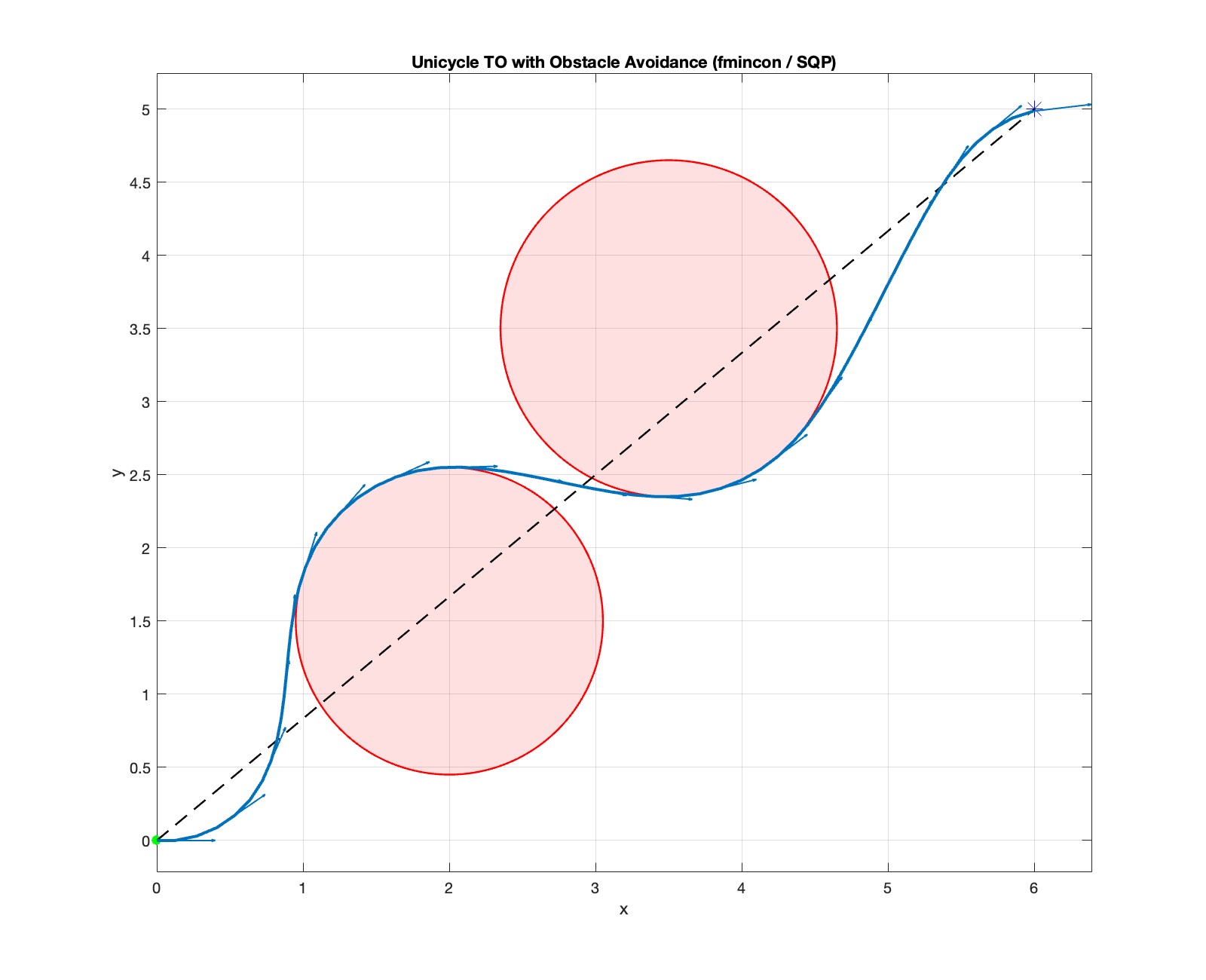
Figure 4.6: Trajectory optimization for unicyle using SQP (two obstacles). Dotted line: initial guess; solid line: optimized trajectory.
Three obstacles (failure). However, when we add a third obstacle, Fig. 4.7 shows that the SQP algorithm converges to an infeasible solution that collides with the obstacles.
You can play with the Matlab code here.
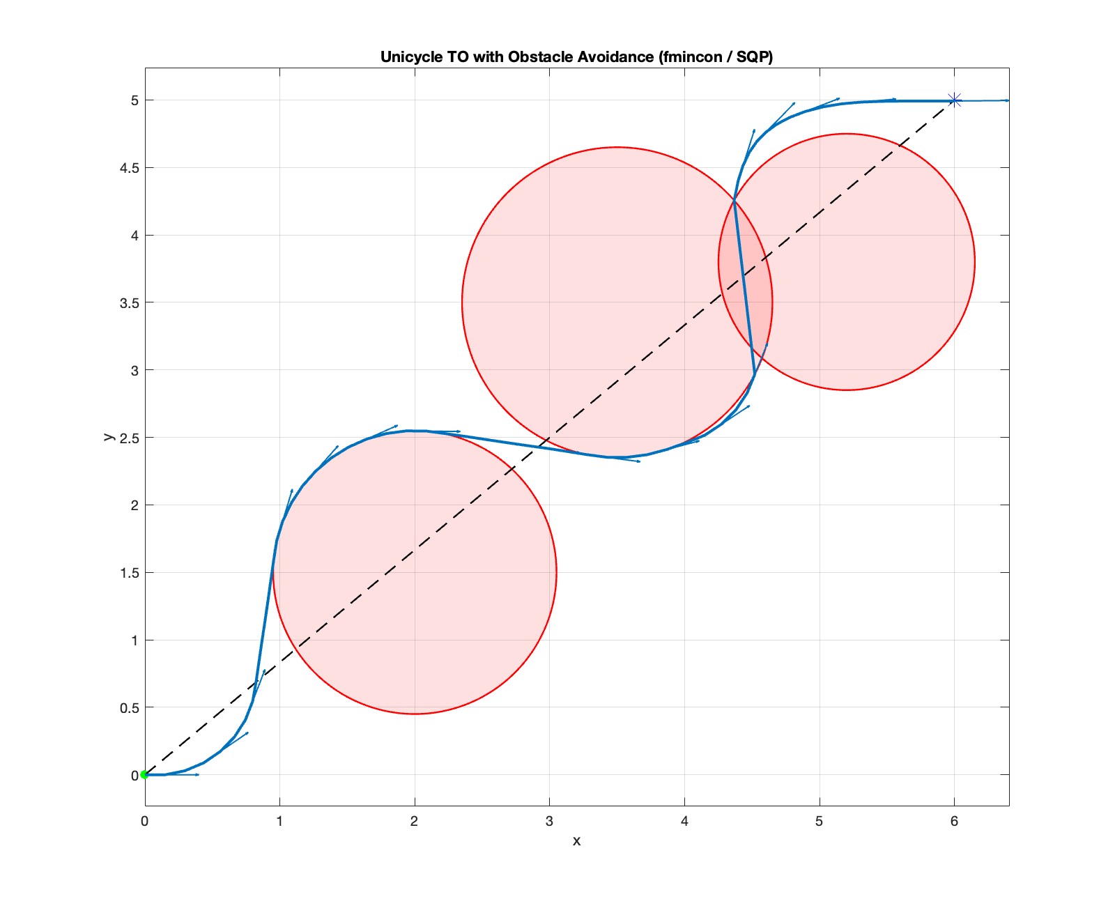
Figure 4.7: Trajectory optimization for unicyle using SQP (three obstacles). Dotted line: initial guess; solid line: optimized trajectory.
The example above highlights both the strengths and the limitations of solving TO with numerical NLP methods such as SQP. Because the TO problem is generally nonconvex, a local method’s outcome depends strongly on the initialization. With a good initial guess, local NLP solvers often converge quickly to a high-quality solution (e.g., Fig. 4.6). With a poor initialization—especially when the landscape has many local minima—the solver may settle in a suboptimal basin or even fail to find a feasible trajectory (e.g., Fig. 4.7).
Global optimization methods can avoid initialization sensitivity and provide global optimality guarantees. These techniques can be substantially more expensive and require additional structure or reformulation, but when applicable they yield powerful initialization-free solutions; see, e.g., (Kang et al. 2024) and references therein.
4.3.5 Interior-Point Methods
We have seen that Primal–Dual Interior-Point Methods (PD-IPM) efficiently solve convex QPs (Section 4.3.3). The key idea was to write the KKT optimality conditions as a system of nonlinear equations and apply Newton’s method. We now extend this idea to the general NLP in (4.55): \[ \min_{x\in\mathbb{R}^n} f(x)\quad\text{s.t.}\quad c(x)=0,\;\; d(x)\le 0, \] where \(f:\mathbb{R}^n \to \mathbb{R}, c:\mathbb{R}^n \to \mathbb{R}^m\) and \(d:\mathbb{R}^n \to\mathbb{R}^p\) are smooth.
4.3.5.1 Lagrangian and KKT
Introduce slack variables \(s\in\mathbb{R}^p\) to convert inequalities to equalities: \[ c(x)=0,\qquad d(x)+s=0,\qquad s\ge 0. \tag{4.66} \]
With equality multipliers \(y\in\mathbb{R}^m, \nu \in \mathbb{R}^p\) and inequality multipliers \(\mu\in\mathbb{R}^p\) (with \(\lambda \ge 0\)), the Lagrangian of the slack-form problem is \[ \mathcal L(x,s,y,\nu,\lambda) \;=\; f(x) + y^\top c(x) + \nu^\top \big(d(x)+s\big) - \lambda^\top s. \tag{4.67} \]
The KKT optimality conditions are (after eliminating \(\nu\)) \[ \begin{aligned} \text{stationarity:}&\quad \nabla f(x) + J_c(x)^\top y + J_d(x)^\top \lambda = 0,\\ \text{primal feasibility:}&\quad c(x)=0,\;\; d(x)+s=0,\;\; s\ge 0,\\ \text{dual feasibility:}&\quad \lambda\ge 0,\\ \text{complementarity:}&\quad s_i\,\lambda_i = 0,\quad i=1,\dots,p, \end{aligned} \tag{4.68} \] where \(J_c=\nabla c(x) \in \mathbb{R}^{m \times n}\), \(J_d=\nabla d(x) \in \mathbb{R}^{p \times n}\).
4.3.5.2 Two Equivalent Views
There are two equivalent ways to derive primal–dual IPMs.
Homotopy / Perturbed KKT (primal–dual view). Replace the complementarity slackness condition in the KKT system (4.68) by a perturbed relation that defines the central path: \[ S\,\lambda \;=\; \mu \,\mathbf{1},\qquad S:=\operatorname{diag}(s),\;\; \mu >0. \tag{4.69} \] Driving the parameter \(\mu \downarrow 0\) yields iterates approaching a KKT point.
Barrier (log-barrier view). Solve the barrier subproblem \[ \min_{x,s>0}\; f(x) - \mu \sum_{i=1}^p \log s_i \quad\text{s.t.}\quad c(x)=0,\;\; d(x)+s=0, \tag{4.70} \] then reduce \(\mu\). The KKT conditions of (4.70) imply \(S\lambda = \mu \mathbf{1}\), hence the barrier and homotopy views are equivalent (different perspectives on the same central path).
4.3.5.3 Primal–Dual Residuals and Newton System
Define residuals at \((x,s,y,\lambda)\): \[ \begin{aligned} r_{\mathrm{dual}} &= \nabla f(x) + J_c^\top y + J_d^\top \lambda,\\ r_{\mathrm{pe}} &= c(x),\\ r_{\mathrm{pi}} &= d(x)+s,\\ r_{\mathrm{cent}} &= S\lambda - \mu \,\mathbf{1}. \end{aligned} \tag{4.71} \] Let \[ H \;:=\; \nabla^2_{xx}\mathcal L(x,s,y,\lambda) = \nabla^2 f(x) + \sum_{i=1}^m y_i \nabla^2 c_i(x) + \sum_{j=1}^p \lambda_j \nabla^2 d_j(x) \tag{4.72} \] be the exact Hessian of the Lagrangian with respect to \(x\).
A primal–dual Newton step \((\Delta x,\Delta s,\Delta y,\Delta \lambda)\) solves \[ \begin{aligned} H\,\Delta x + J_c^\top \Delta y + J_d^\top \Delta \lambda &= -\,r_{\mathrm{dual}},\\ J_c\,\Delta x &= -\,r_{\mathrm{pe}},\\ J_d\,\Delta x + \Delta s &= -\,r_{\mathrm{pi}},\\ S\,\Delta \lambda + M\,\Delta s &= -\,r_{\mathrm{cent}},\qquad M:=\operatorname{diag}(\lambda). \end{aligned} \tag{4.73} \]
Eliminating \(\Delta s=-r_{\mathrm{pi}}-J_d\Delta x\) gives \[ \Delta \lambda = S^{-1}\!\left(-r_{\mathrm{cent}} + M\,r_{\mathrm{pi}} + M\,J_d\,\Delta x\right). \tag{4.74} \] Substitute into the first line to obtain the reduced symmetric system in \((\Delta x,\Delta y)\): \[ \begin{bmatrix} H + J_d^\top D\,J_d & J_c^\top\\[2pt] J_c & 0 \end{bmatrix} \begin{bmatrix}\Delta x\\ \Delta y\end{bmatrix} = - \begin{bmatrix} r_{\mathrm{dual}} + J_d^\top S^{-1}\!\big(-r_{\mathrm{cent}} + M r_{\mathrm{pi}}\big)\\[2pt] r_{\mathrm{pe}} \end{bmatrix} \tag{4.75} \] with \(D:=S^{-1}M\). Then recover \(\Delta \lambda\) via (4.74) and \(\Delta s=-r_{\mathrm{pi}}-J_d\Delta x\).
4.3.5.4 Line-search IPM
Step lengths (fraction-to-the-boundary). Choose positive step sizes that keep strict interiority: \[ \alpha_{\mathrm{pri}}=\min\!\Big(1,\ \eta \min_{\Delta s_i<0}\frac{-s_i}{\Delta s_i}\Big),\quad \alpha_{\mathrm{du}} =\min\!\Big(1,\ \eta \min_{\Delta \lambda_i<0}\frac{-\lambda_i}{\Delta \lambda_i}\Big),\quad \eta\in(0,1). \tag{4.76} \]
Merit (or filter) globalization. Use a barrier merit for backtracking, \[ \Phi_{\mu}(x,s) \;=\; f(x) - \mu \sum_i \log s_i + \frac{\rho}{2}\,\|c(x)\|_2^2 + \frac{\rho}{2}\,\|d(x)+s\|_2^2, \tag{4.77} \] or a filter that accepts steps reducing either infeasibility or the barrier objective.
Mehrotra predictor–corrector (recommended).
Predictor (affine) step: solve (4.75) with \(\mu=0\) to get \((\Delta x^{\mathrm{aff}},\Delta s^{\mathrm{aff}},\Delta y^{\mathrm{aff}},\Delta\lambda^{\mathrm{aff}})\), and affine step sizes \(\alpha_{\mathrm{pri}}^{\mathrm{aff}},\alpha_{\mathrm{du}}^{\mathrm{aff}}\).
Centering: set \[ \tau_{\mathrm{aff}}=\frac{(s+\alpha_{\mathrm{pri}}^{\mathrm{aff}}\Delta s^{\mathrm{aff}})^\top (\lambda+\alpha_{\mathrm{du}}^{\mathrm{aff}}\Delta\lambda^{\mathrm{aff}})}{p},\qquad \sigma=\left(\frac{\tau_{\mathrm{aff}}}{\frac{s^\top\mu}{p}}\right)^{3}, \] and replace the complementarity RHS by \(\mu=\sigma\,\frac{s^\top\lambda}{p}\).
Corrector: resolve (4.75) with the corrected central residual \[ r_{\mathrm{cent}}^{\mathrm{corr}} = S\lambda - \mu \,\mathbf{1} - \Delta S^{\mathrm{aff}}\Delta\lambda^{\mathrm{aff}}\mathbf{1}. \tag{4.78} \]
Line search & update: use (4.76) and backtrack on \(\Phi_{\mu}\).
Stopping: terminate inner loop when \(\|r_{\mathrm{dual}}\|_\infty,\|r_{\mathrm{pe}}\|_\infty,\|r_{\mathrm{pi}}\|_\infty\) and the average complementarity \(\frac{s^\top\mu}{p}\) are below tolerance; then reduce \(\mu\) and repeat.
Hessian Modeling. Use \(H=\nabla^2_{xx}\mathcal L\), or a damped (L-)BFGS / Gauss–Newton model as in Section 4.3.4.4.
4.3.5.5 Trust-Region IPM
The trust-region (TR) IPM solves the barrier subproblem (4.70) inexactly within a TR globalization that is scaled to the slacks to avoid steps that approach the boundary too aggressively.
The TR-IPM subproblem is the local quadratic model of the barrier problem together with a metric that respects distance to the boundary.
Quadratic model of the barrier objective. Start from the barrier problem \[ \min_{x,s>0}\ f(x)-\mu\sum_i\log s_i \quad\text{s.t.}\quad c(x)=0,\ d(x)+s=0. \] A second-order Taylor model at \((x,s)\) gives (constants omitted) \[ m(p_x,p_s)\;\approx\; \nabla f^\top p_x+\frac{1}{2} p_x^\top H\,p_x \;-\;\mu\,\mathbf 1^\top S^{-1}p_s \;+\;\frac{1}{2}\,\mu\,\|S^{-1}p_s\|_2^2, \] where \(H=\nabla^2_{xx}\mathcal L\) and \(S=\operatorname{diag}(s)\). The linear term \(-\mu\,\mathbf1^\top S^{-1}p_s\) is exactly the gradient of the log-barrier in the slack coordinates. The quadratic curvature in \(p_s\) is \(\mu S^{-2}\).
Many implementations move (part of) this curvature into the TR metric, replacing the explicit \(+\frac{1}{2}\,\mu\|S^{-1}p_s\|^2\) by the scaled trust region below. This avoids double-counting and makes the subproblem simpler while keeping the right geometry.
Linearized constraints for a consistent local step.
\[ J_c\,p_x + c(x)=0,\qquad J_d\,p_x + p_s + d(x)=0. \] These are the first-order feasibility conditions of the barrier constraints.Scaled trust region \(\| (p_x,\;S^{-1}p_s)\|\le \Delta\). The scaling by \(S^{-1}\) measures \(p_s\) relative to the current distance to the boundary. If a slack \(s_i\) is tiny, even a small absolute change \(p_{s,i}\) is risky; the scaled norm automatically shrinks the allowable step in that direction. This yields:
- Boundary awareness: steps cannot run into \(s_i\le0\) unless the trust region is (incorrectly) large.
- Scale invariance: the step is insensitive to units or simple rescalings of the inequalities.
- Numerical stability: the local subproblem remains well conditioned near the boundary.
- Boundary awareness: steps cannot run into \(s_i\le0\) unless the trust region is (incorrectly) large.
Fraction-to-the-boundary safeguard \(p_s\ge -\tau s\). This is a simple interiority constraint ensuring \(s+\alpha p_s>0\) for admissible step sizes.
Putting these choices together yields the subproblem \[ \min_{p_x,p_s}\ \nabla f^\top p_x+\frac{1}{2} p_x^\top H p_x - \mu\,\mathbf1^\top S^{-1}p_s \quad\text{s.t.}\quad \begin{cases} J_c p_x + c(x)=0,\\ J_d p_x + p_s + d(x)=0,\\ \|(p_x,S^{-1}p_s)\|\le\Delta,\ p_s\ge-\tau s, \end{cases} \tag{4.79} \] which is exactly a trust-region SQP step on the barrier problem in the barrier metric.
The outer loop adapts the trust-region radius \(\Delta\) and the barrier parameter \(\mu\) as follows.
- Updating \(\Delta\) (model–reality agreement). After computing a trial step \(p=(p_x,p_s)\) from the scaled TR subproblem (4.79), compare the predicted reduction from the quadratic model to the actual reduction in the barrier merit:
\[
\rho \;=\; \frac{\text{ared}}{\text{pred}}
\;=\;
\frac{\Phi_\mu(x,s)-\Phi_\mu(x+p_x,\,s+p_s)}
{\text{model}(0)-\text{model}(p)}.
\]
With thresholds \(0<\eta_1<\eta_2<1\) and factors \(\gamma_{\text{dec}}\in(0,1)\), \(\gamma_{\text{inc}}>1\):
- If \(\rho\ge \eta_2\): accept the step and enlarge the radius, \(\Delta \leftarrow \min(\gamma_{\text{inc}}\Delta,\Delta_{\max})\).
- If \(\eta_1 \le \rho < \eta_2\): accept and keep \(\Delta\).
- If \(\rho<\eta_1\): reject the step and shrink the radius, \(\Delta \leftarrow \gamma_{\text{dec}}\Delta\), then resolve the TR subproblem.
- Updating \(\mu\) (centrality progress). Decrease the barrier parameter \(\mu\) only when the current barrier subproblem is solved to an accuracy commensurate with \(\mu\). Using KKT residuals and average complementarity \[ \tau \;:=\; \frac{s^\top \lambda}{p}, \] require (for some constants \(\kappa_{\rm dual},\kappa_{\rm pe},\kappa_{\rm pi},\kappa_{\rm cent}>0\)) \[ \|r_{\rm dual}\|_\infty \le \kappa_{\rm dual}\,\mu,\quad \|r_{\rm pe}\|_\infty \le \kappa_{\rm pe}\,\mu,\quad \|r_{\rm pi}\|_\infty \le \kappa_{\rm pi}\,\mu,\quad |\tau-\mu| \le \kappa_{\rm cent}\,\mu. \] When these hold, reduce \(\mu\) (e.g., \(\mu\leftarrow\theta\,\mu\) with \(\theta\in(0,1)\)). If the tests are not met, hold \(\mu\) fixed and continue improving the inner TR solve (possibly with an updated \(\Delta\)).
When to favor TR-IPM. TR globalization is robust for nonconvex \(H\), allows inexact linear solves (e.g., Krylov), and integrates naturally with limited-memory updates and scaling.
Software. Implementing a robust interior-point method that reliably solves general nonlinear programs is nontrivial. Fortunately, the open-source solver IPOPT (Wächter and Biegler 2006) is a mature, widely used option that exploits sparsity and supports exact or quasi-Newton Hessians. In what follows, we formulate a trajectory-optimization problem and solve it with IPOPT to illustrate end-to-end modeling and solver usage.
Example 4.5 (Trajectory Optimization with IPOPT) We solve a unicycle trajectory optimization (TO) problem (same as the one in Example 4.4) from start pose \(A\) to goal pose \(B\) while avoiding circular obstacles, now using IPOPT via cyipopt in Python.
Dynamics. With state \(x=[p_x,p_y,\theta]^\top\) and control \(u=[v,\omega]^\top\), \[ \dot{x}(t)= \begin{bmatrix} v\cos\theta\\[2pt] v\sin\theta\\ \omega \end{bmatrix}. \tag{4.80} \] We discretize at \(t_k=kh\) by forward Euler: \[ x_{k+1} = f_h(x_k,u_k) := \begin{bmatrix} p_{x,k} + h\, v_k \cos \theta_k\\ p_{y,k} + h\, v_k \sin \theta_k\\ \theta_k + h\, \omega_k \end{bmatrix},\quad k=0,\ldots,N-1. \tag{4.81} \]
Decision vector. We stack the state and control trajectories into a single decision vector \[ z=\big[x_0^\top,u_0^\top,x_1^\top,u_1^\top,\dots,x_{N-1}^\top,u_{N-1}^\top,x_N^\top\big]^\top \in\mathbb{R}^{(3+2)N+3}. \tag{4.82} \]
Constraints. The state and control trajectories need to satisfy the following constraints:
Initial condition: \(x_0=A\).
Dynamics equalities: \(x_{k+1}-f_h(x_k,u_k)=0\) for \(k=0,\dots,N-1\).
Obstacle inequalities: for each circular obstacle \((c_j=[c_{x,j},c_{y,j}]^\top,r_j)\) and all \(k=0,\dots,N\), \[ c_{j,k}(x_k):=(r_j+\delta)^2-\big((p_{x,k}-c_{x,j})^2+(p_{y,k}-c_{y,j})^2\big)\le 0, \tag{4.83} \] where \(\delta > 0\) is a safety margin.
Box bounds on controls: \[ v_{\min}\le v_k\le v_{\max},\qquad \omega_{\min}\le \omega_k\le \omega_{\max}. \tag{4.84} \]
In total, there are \(m = 3 + 3N\) equality constraints and \(p = (N+1)O\) inequality constraints, where \(O\) is the number of obstacles.
Objective. A smooth quadratic cost with terminal goal tracking, control effort, and control smoothness: \[\begin{equation} \hspace{-16mm} J = \frac12\Big( w_{\text{pos}}\|x_N^{\text{pos}}-B^{\text{pos}}\|_2^2 + w_\theta(\theta_N-\theta^\star)^2 + \sum_{k=0}^{N-1} w_u \|u_k\|_2^2 + \sum_{k=0}^{N-2} w_{\Delta u}\|u_{k+1}-u_k\|_2^2 \Big), \tag{4.85} \end{equation}\] with \(x_N^{\text{pos}}=[p_{x,N},p_{y,N}]^\top\) the terminal position and \(B=[B_x,B_y,\theta^\star]^\top\) the terminal pose. \(w_{\text{pos}}\), \(w_\theta\), \(w_u\), and \(w_{\Delta u}\) are positive weights.
Jacobians. We derive the gradient of the objective and the Jacobian of the constraints with respect to the stacked decision vector \[ z \;=\; \big[x_0^\top,\ u_0^\top,\ x_1^\top,\ u_1^\top,\ \dots,\ x_{N-1}^\top,\ u_{N-1}^\top,\ x_N^\top\big]^\top \in \mathbb{R}^{(3+2)N+3}, \] where \(x_k=[p_{x,k},\,p_{y,k},\,\theta_k]^\top\) and \(u_k=[v_k,\,\omega_k]^\top\).
Objective gradient \(\nabla_z J\). Recall the objective function from (4.85). Let \(e_{\text{pos}} := x_N^{\text{pos}}-B^{\text{pos}}\) and \(e_\theta := \theta_N-\theta^\star\), we have \[ \frac{\partial J}{\partial p_{x,N}} = w_{\text{pos}}\, e_{\text{pos},x},\qquad \frac{\partial J}{\partial p_{y,N}} = w_{\text{pos}}\, e_{\text{pos},y},\qquad \frac{\partial J}{\partial \theta_N} = w_\theta\, e_\theta. \]
All other states \(x_k\) for \(k<N\) do not appear in the objective, so \[ \frac{\partial J}{\partial x_k} = 0,\quad k=0,\dots,N-1. \]
The control effort term in the objective has gradients w.r.t. controls: \[ J_u \;=\; \frac{1}{2}\sum_{k=0}^{N-1} w_u \| u_k \|^2 \Rightarrow\; \frac{\partial J_u}{\partial u_k} \;=\; w_u\,u_k \quad\text{for }k=0,\dots,N-1. \]
The control smoothness term in the objective reads: \[ J_{\Delta u} \;=\; \frac{1}{2}\sum_{k=0}^{N-2} w_{\Delta u}\,\|u_{k+1}-u_k\|_2^2. \] By collecting contributions from the two adjacent differences that contain \(u_k\), we obtain the gradient \[ \frac{\partial J_{\Delta u}}{\partial u_k} = \begin{cases} w_{\Delta u}\,(u_0 - u_1), & k=0,\\[4pt] w_{\Delta u}\,(2u_k - u_{k-1} - u_{k+1}), & k=1,\dots,N-2,\\[4pt] w_{\Delta u}\,(u_{N-1} - u_{N-2}), & k=N-1. \end{cases} \tag{4.86} \]
Combining the above derivations, the only nonzero blocks of \(\nabla_z J\) are:
the terminal state block \(x_N\): entries shown above for \(p_{x,N},p_{y,N},\theta_N\);
the control blocks \(u_k\): \(w_u u_k\) plus the smoothness terms (4.86).
All other entries are zero. Thus \(\nabla_z J\) is extremely sparse.
Constraint Jacobian \(\nabla_z g(z)\). We stack constraints as \[ g(z)=\begin{bmatrix} g^{\text{init}}\\ g^{\text{dyn}}\\ g^{\text{obs}} \end{bmatrix} \in \mathbb{R}^{3+3N+(N+1)O} \] in the order:
Initial condition \(g^{\text{init}} = x_0 - A = 0\).
Dynamics for \(k=0,\dots,N-1\) (forward Euler with step \(h\)): \[ \begin{aligned} g^{\text{dyn}}_{x,k}&:= p_{x,k+1} - \big(p_{x,k} + h\,v_k\cos\theta_k\big) = 0,\\ g^{\text{dyn}}_{y,k}&:= p_{y,k+1} - \big(p_{y,k} + h\,v_k\sin\theta_k\big) = 0,\\ g^{\text{dyn}}_{\theta,k}&:= \theta_{k+1} - \big(\theta_k + h\,\omega_k\big) = 0. \end{aligned} \]
Obstacle inequalities for each obstacle \(j=1,\dots,O\) and each knot \(k=0,\dots,N\): \[ g^{\text{obs}}_{j,k} \;:=\; (r_j+\delta)^2 - \Big((p_{x,k}-c_{x,j})^2 + (p_{y,k}-c_{y,j})^2\Big) \;\le\; 0. \]
Below we list nonzero partial derivatives; all missing entries are \(0\).
(i) Initial condition \(g^{\text{init}}=x_0-A\) \[ \frac{\partial g^{\text{init}}}{\partial x_0} = I_3. \]
(ii) Dynamics rows at time \(k\)
\(x\)-row \(g^{\text{dyn}}_{x,k}\): \[ \frac{\partial g^{\text{dyn}}_{x,k}}{\partial p_{x,k+1}}=1,\quad \frac{\partial g^{\text{dyn}}_{x,k}}{\partial p_{x,k}}=-1,\quad \frac{\partial g^{\text{dyn}}_{x,k}}{\partial \theta_k}=h\,v_k\sin\theta_k,\quad \frac{\partial g^{\text{dyn}}_{x,k}}{\partial v_k}=-h\cos\theta_k. \]
\(y\)-row \(g^{\text{dyn}}_{y,k}\): \[ \frac{\partial g^{\text{dyn}}_{y,k}}{\partial p_{y,k+1}}=1,\quad \frac{\partial g^{\text{dyn}}_{y,k}}{\partial p_{y,k}}=-1,\quad \frac{\partial g^{\text{dyn}}_{y,k}}{\partial \theta_k}=-h\,v_k\cos\theta_k,\quad \frac{\partial g^{\text{dyn}}_{y,k}}{\partial v_k}=-h\sin\theta_k. \]
Heading row \(g^{\text{dyn}}_{\theta,k}\): \[ \frac{\partial g^{\text{dyn}}_{\theta,k}}{\partial \theta_{k+1}}=1,\quad \frac{\partial g^{\text{dyn}}_{\theta,k}}{\partial \theta_k}=-1,\quad \frac{\partial g^{\text{dyn}}_{\theta,k}}{\partial \omega_k}=-h. \]
All other partials in each row are zero. Each dynamics triple only touches the local block \((x_k,u_k,x_{k+1})\), yielding a banded, block-sparse Jacobian in time.
(iii) Obstacle row for \((j,k)\) \[ g^{\text{obs}}_{j,k}=(r_j+\delta)^2 - \big((p_{x,k}-c_{x,j})^2+(p_{y,k}-c_{y,j})^2\big). \] Nonzeros: \[ \frac{\partial g^{\text{obs}}_{j,k}}{\partial p_{x,k}}=-2\,(p_{x,k}-c_{x,j}),\qquad \frac{\partial g^{\text{obs}}_{j,k}}{\partial p_{y,k}}=-2\,(p_{y,k}-c_{y,j}). \] This row depends only on the position of \(x_k\), so each obstacle row touches exactly two columns \((p_{x,k},p_{y,k})\).
Combining the derivations above, we can see the Jacobian \(\nabla_z g\) is block-banded in time.
Initial block at \(x_0\) is identity.
Each dynamics row touches \((x_k, u_k, x_{k+1})\) with at most 4 nonzeros in the \(x\)- and \(y\)-rows and 3 nonzeros in the \(\theta\)-row.
Each obstacle row touches only \((p_{x,k}, p_{y,k})\).
Fig. 4.8 illustrates the sparsity structure of the constraint Jacobian.
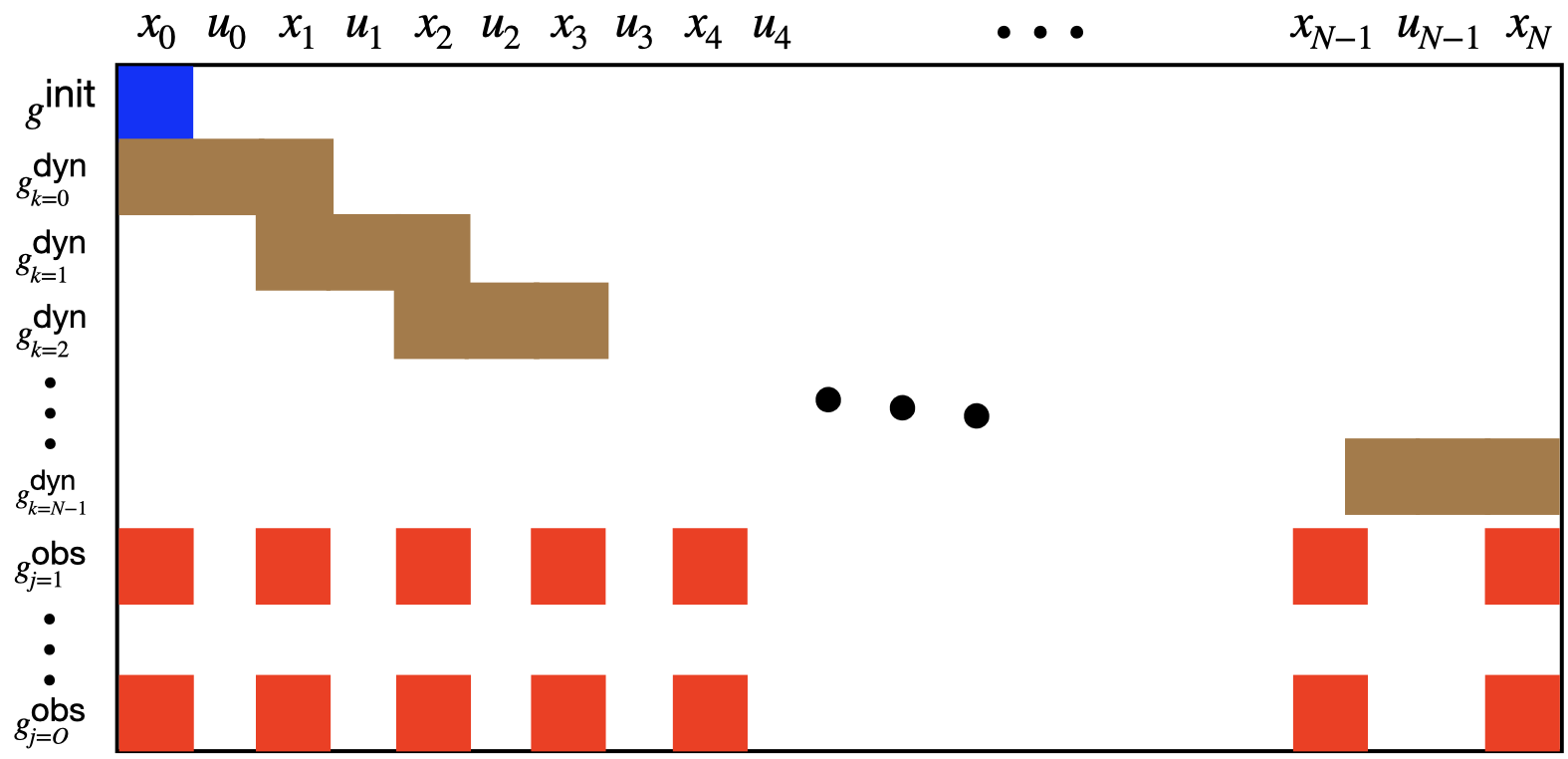
Figure 4.8: Sparsity structure of constraint Jacobian.
The following Python code snippet defines a problem class UnicycleTO with definitions of the objective, constraints, objective gradient, and constraints Jacobian. Note that the definition of the constraints Jacobian is highly involved because it defines the Jacobian as a sparse matrix with a predefined sparsity pattern. The solver can leverage this sparsity pattern to be highly efficient.
class UnicycleTO:
    def __init__(self, P: Params):
        self.P = P
        # --- Build bounds on variables ---
        lb = -np.inf * np.ones(P.Z_DIM)
        ub =  np.inf * np.ones(P.Z_DIM)
        for k in range(P.N):
            iu = idx_u(k, P)
            lb[iu.start + 0] = P.v_min
            ub[iu.start + 0] = P.v_max
            lb[iu.start + 1] = P.w_min
            ub[iu.start + 1] = P.w_max
        self.lb = lb
        self.ub = ub

        # --- Build bounds on constraints ---
        cl = np.zeros(P.M)
        cu = np.zeros(P.M)
        # equalities: exactly 0
        cl[:P.n_ceq] = 0.0
        cu[:P.n_ceq] = 0.0
        # inequalities: c <= 0
        cl[P.n_ceq:] = -np.inf
        cu[P.n_ceq:] = 0.0
        self.cl = cl
        self.cu = cu

        # --- Precompute Jacobian sparsity (row, col) ---
        self.jac_rows, self.jac_cols = self._build_jacobian_structure()

    # Objective
    def objective(self, z):
        P = self.P
        X, U = unpack(z, P)

        # Terminal goal tracking
        pos_err = X[-1, 0:2] - P.B[0:2]
        th_err  = X[-1, 2]   - P.B[2]
        J_goal = P.w_goal_pos * np.dot(pos_err, pos_err) + P.w_goal_theta * (th_err**2)

        # Control effort
        J_u = P.w_u * np.sum(U * U)

        # Control smoothness
        dU = U[1:, :] - U[:-1, :]
        J_du = P.w_du * np.sum(dU * dU)

        return 0.5 * (J_goal + J_u + J_du)

    # Gradient of objective
    def gradient(self, z):
        P = self.P
        X, U = unpack(z, P)
        grad = np.zeros(P.Z_DIM)

        # Terminal contributions (no 0.5 after derivative: cancels 2)
        pos_err = X[-1, 0:2] - P.B[0:2]
        th_err  = X[-1, 2]   - P.B[2]
        gN = np.array([P.w_goal_pos * pos_err[0],
                       P.w_goal_pos * pos_err[1],
                       P.w_goal_theta * th_err])
        grad[idx_x(P.N, P)] += gN

        # Control effort: 0.5 * 2 * w_u * u = w_u * u
        for k in range(P.N):
            iu = idx_u(k, P)
            grad[iu] += P.w_u * U[k, :]

        # Control smoothness: 0.5 * w_du * sum ||u_{k+1}-u_k||^2
        # d/d u_k:   -w_du*(u_{k+1}-u_k)  from (k,k+1)
        # d/d u_{k+1}: +w_du*(u_{k+1}-u_k)
        for k in range(P.N - 1):
            du = U[k + 1, :] - U[k, :]
            grad[idx_u(k, P)]     += -P.w_du * du
            grad[idx_u(k + 1, P)] +=  P.w_du * du

        return grad

    # Constraints g(z)
    def constraints(self, z):
        P = self.P
        X, U = unpack(z, P)
        g = np.zeros(P.M)
        r = 0

        # Initial equality: X0 - A = 0
        g[r:r+3] = X[0, :] - P.A
        r += 3

        # Dynamics equalities
        for k in range(P.N):
            xk = X[k, :]
            uk = U[k, :]
            xnext = f_disc(xk, uk, P.h)
            g[r:r+3] = X[k + 1, :] - xnext
            r += 3

        # Obstacle inequalities: (r+margin)^2 - ((px-cx)^2 + (py-cy)^2) <= 0
        for k in range(P.N + 1):
            px, py = X[k, 0], X[k, 1]
            for j in range(P.nObs):
                cx, cy, r0 = P.obstacles[j]
                r_eff = r0 + P.safety_margin
                g[r] = (r_eff ** 2) - ((px - cx) ** 2 + (py - cy) ** 2)
                r += 1

        return g

    # Jacobian sparsity
    def jacobianstructure(self):
        return (np.array(self.jac_rows, dtype=int),
                np.array(self.jac_cols, dtype=int))

    # Jacobian values (in the same order as jacobianstructure)
    def jacobian(self, z):
        P = self.P
        X, U = unpack(z, P)
        vals = []
        r = 0

        # Initial eq: d/dX0 is identity (one per row)
        # rows r..r+2 with columns X0(px,py,th)
        for i in range(3):
            vals.append(1.0)
        r += 3

        # Dynamics eqs
        for k in range(P.N):
            xk = X[k, :]
            uk = U[k, :]
            th = xk[2]
            v  = uk[0]

            # Row r: g1 = x_{k+1,px} - [px_k + h v cos(th_k)]
            # d wrt X_{k+1,px}
            vals.append(1.0)
            # d wrt X_k,px
            vals.append(-1.0)
            # d wrt X_k,theta ( + h v sin(th) )
            vals.append(P.h * v * np.sin(th))
            # d wrt U_k,v ( - h cos(th) )
            vals.append(-P.h * np.cos(th))

            # Row r+1: g2 = x_{k+1,py} - [py_k + h v sin(th_k)]
            vals.append(1.0)                  # d wrt X_{k+1,py}
            vals.append(-1.0)                 # d wrt X_k,py
            vals.append(-P.h * v * np.cos(th))# d wrt X_k,theta
            vals.append(-P.h * np.sin(th))    # d wrt U_k,v

            # Row r+2: g3 = x_{k+1,th} - [th_k + h w_k]
            vals.append(1.0)   # d wrt X_{k+1,theta}
            vals.append(-1.0)  # d wrt X_k,theta
            vals.append(-P.h)  # d wrt U_k,omega

            r += 3

        # Obstacle inequalities
        for k in range(P.N + 1):
            px, py = X[k, 0], X[k, 1]
            for j in range(P.nObs):
                cx, cy, _ = P.obstacles[j]
                # d/d px_k: -2(px - cx)
                vals.append(-2.0 * (px - cx))
                # d/d py_k: -2(py - cy)
                vals.append(-2.0 * (py - cy))
                r += 1

        return np.array(vals, dtype=float)

    # --- Internal: build Jacobian sparsity pattern once ---
    def _build_jacobian_structure(self):
        P = self.P
        rows = []
        cols = []
        r = 0

        # Initial equality: g0..g2 depend on X0(px,py,th) diagonally
        for i in range(3):
            rows.append(r + i)
            cols.append(idx_x(0, P).start + i)
        r += 3

        # Dynamics equalities
        for k in range(P.N):
            ixk   = idx_x(k, P)
            ixkp1 = idx_x(k + 1, P)
            iuk   = idx_u(k, P)

            # Row r (px)
            rows.extend([r, r, r, r])
            cols.extend([
                ixkp1.start + 0,   # X_{k+1,px}
                ixk.start   + 0,   # X_k,px
                ixk.start   + 2,   # X_k,theta
                iuk.start   + 0    # U_k,v
            ])
            # Row r+1 (py)
            rows.extend([r + 1, r + 1, r + 1, r + 1])
            cols.extend([
                ixkp1.start + 1,   # X_{k+1,py}
                ixk.start   + 1,   # X_k,py
                ixk.start   + 2,   # X_k,theta
                iuk.start   + 0    # U_k,v
            ])
            # Row r+2 (theta)
            rows.extend([r + 2, r + 2, r + 2])
            cols.extend([
                ixkp1.start + 2,   # X_{k+1,theta}
                ixk.start   + 2,   # X_k,theta
                iuk.start   + 1    # U_k,omega
            ])
            r += 3

        # Obstacle inequalities: each depends only on px_k, py_k
        for k in range(P.N + 1):
            ixk = idx_x(k, P)
            for _ in range(P.nObs):
                rows.extend([r, r])
                cols.extend([ixk.start + 0, ixk.start + 1])
                r += 1

        assert r == P.M, "Jacobian structure row count mismatch"
        return rows, cols
After defining the problem class, we pass it to the interface of IPOPT using the folowing snippet.
# Initial guess
z0 = initial_guess(P)

# Problem + IPOPT
problem = UnicycleTO(P)
nlp = cyipopt.Problem(
    n=P.Z_DIM, m=P.M,
    problem_obj=problem,
    lb=problem.lb, ub=problem.ub,
    cl=problem.cl, cu=problem.cu
)

# Options (tweak as desired)
nlp.add_option("tol", 1e-6)
nlp.add_option("dual_inf_tol", 1e-6)
nlp.add_option("constr_viol_tol", 1e-6)
nlp.add_option("compl_inf_tol", 1e-6)
nlp.add_option("max_iter", 2000)
nlp.add_option("hessian_approximation", "limited-memory")
nlp.add_option("print_level", 5)

z_star, info = nlp.solve(z0)
In the case of three obstacles (\(\delta=0\)), we obtain the trajectory shown in Fig. 4.9 with an all-zero initialization; the trajectory shown in Fig. 4.10 with a straight-line initialization; and the trajectory shown in Fig. @ref(fig: unicycle-to-ipopt-random) with a random initialization.
You can play with the full code here.
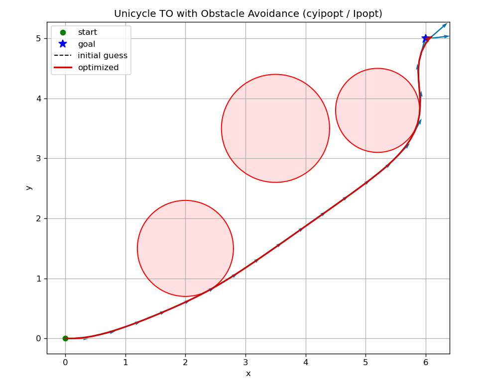
Figure 4.9: Trajectory optimization for unicyle using IPOPT (all-zero initialization).
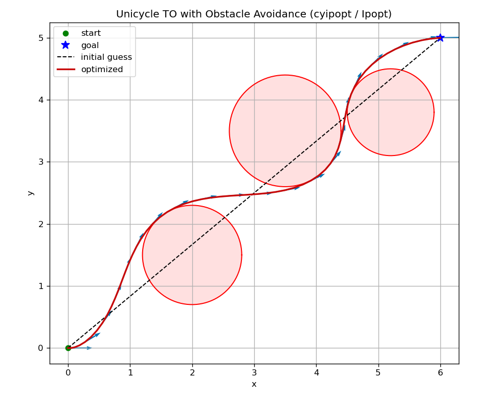
Figure 4.10: Trajectory optimization for unicyle using IPOPT (straight-line initialization).
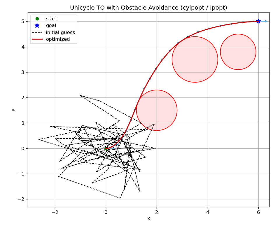
Figure 4.11: Trajectory optimization for unicyle using IPOPT (random initialization).
4.4 Model Predictive Control
Trajectory optimization (TO) computes (locally or globally) optimal trajectories that are dynamically feasible with respect to a chosen discrete-time transcription and satisfy system constraints at the discretization grid. As a consequence, the resulting plan is open loop: it neither accounts for disturbances nor provides feedback. A common remedy is LQR trajectory tracking (Section 4.2), which linearizes the dynamics along the nominal trajectory to synthesize a local feedback controller. While effective near the nominal path, this approach can struggle in the presence of obstacles or whenever the reference trajectory itself must change over time.
Model predictive control (MPC) addresses these limitations by turning TO into a receding-horizon feedback policy. At each control step, MPC resolves a finite-horizon optimal control problem with the current measured state as the initial condition, applies only the first control action, and then repeats the procedure at the next step. This closes the loop, providing robustness to model mismatch and disturbances while naturally adapting the trajectory as the environment or task evolves. In this section we introduce the core ideas behind MPC; for a comprehensive treatment, see (Rawlings, Mayne, and Diehl 2020).
Dynamics. Let us consider a discrete-time dynamical system \[\begin{equation} s_{t+1} = f(s_t, a_t, w_t), \tag{4.87} \end{equation}\] where \(s_t \in \mathbb{R}^n\) represents the state, \(a_t \in \mathbb{R}^m\) represents the control/action, and \(w_t \in \mathbb{R}^d\) represents a stochastic disturbance. With slight abuse of notation, let us use \[ s_{t+1} = f (s_t, a_t) \equiv f (s_t, a_t, 0) \] to denote the system dynamics without the disturbance.
Here we have used \((s_t, a_t)\) to represent the state and control. This departs from the notation (4.1) used in the beginning. The reason for doing so will become clear soon.
Trajectory Optimization. At time step \(t\), let the system’s state be \(s_t\) as given (e.g., measured from sensor data). MPC solves the following open-loop TO problem, adapted from (4.29): \[\begin{equation} \begin{split} \min_{\{x_k,u_k\}} \quad & \Phi(x_N) + \sum_{k=0}^{N-1} \ell_k(x_k,u_k) \\[2mm] \text{s.t.}\quad & x_{k+1} = f (x_k,u_k), \qquad t=0,\dots,N-1,\\ & \boxed{x_0 = s_t} \ \ \text{(given)},\\ & x_k \in \mathcal X_k,\quad u_k \in \mathcal U_k \quad \text{(bounds)},\\ & g_k(x_k,u_k) \le 0,\quad h_k(x_k,u_k)=0 \quad \text{(path/terminal constraints).} \end{split} \tag{4.88} \end{equation}\] Notice that in (4.88):
We used \(k\) to denote the time step in the TO problem, in contrast to \(t\) in the system dynamics.
We used \((x_k,u_k)\) to denote the state and control in the TO problem, as opposed to \((s_t, a_t)\) in the system dynamics.
We enforce the TO problem starts at \(x_0 = s_t\), i.e., the initial state in trajectory planning aligns with the current system state at time \(t\).
Receding Horizon Control. Let \[\begin{equation} (x_0^\star, u_0^\star, x_1^\star, u_1^\star, \dots, x_{N-1}^\star, u_{N-1}^\star, x_N^\star) \tag{4.89} \end{equation}\] be an optimal solution of the TO problem (4.88) (e.g., obtained from IPOPT). Instead of executing the entire sequence of optimal controls \((u_0^\star, u_1^\star, \dots, u_{N-1}^\star)\), MPC will only execute the first element. Formally, the actual control action applied to the system, denoted as \(a_t\), is \[\begin{equation} a_t = u_0^\star. \tag{4.90} \end{equation}\] Applying \(a_t = u_0^\star\) to the real dynamics (4.87), the system will step into a new state \(s_{t+1}\) at time \(t+1\): \[ s_{t+1} = f(s_t, u_0^\star, w_t). \] Then, MPC solves a new TO problem that is exactly the same as the problem (4.88) at time \(t\), except that the initial state is changed to \(s_{t+1}\): \[\begin{equation} \begin{split} \min_{\{x_k,u_k\}} \quad & \Phi(x_N) + \sum_{k=0}^{N-1} \ell_k(x_k,u_k) \\[2mm] \text{s.t.}\quad & x_{k+1} = f (x_k,u_k), \qquad t=0,\dots,N-1,\\ & \boxed{x_0 = s_{t+1}} \ \ \text{(given)},\\ & x_k \in \mathcal X_k,\quad u_k \in \mathcal U_k \quad \text{(bounds)},\\ & g_k(x_k,u_k) \le 0,\quad h_k(x_k,u_k)=0 \quad \text{(path/terminal constraints).} \end{split} \tag{4.91} \end{equation}\] Problems (4.88) and (4.91) are called parametric optimization problems, in the sense that the form of the optimization problem remains the same, but the value of the parameter \(s_t\) that defines the equality constraint has changed.
For this reason, we should restate the solution in (4.89) as \[\begin{equation} (x_0^\star(s_t), u_0^\star(s_t), x_1^\star(s_t), u_1^\star(s_t), \dots, x_{N-1}^\star(s_t), u_{N-1}^\star(s_t), x_N^\star(s_t)) \tag{4.92} \end{equation}\] because they are all implicit functions of the parameter \(s_t\).
Similarly, the solution to the TO problem (4.91) at time \(t+1\) should be denoted as \[\begin{equation} (x_0^\star(s_{t+1}), u_0^\star(s_{t+1}), x_1^\star(s_{t+1}), u_1^\star(s_{t+1}), \dots, x_{N-1}^\star(s_{t+1}), u_{N-1}^\star(s_{t+1}), x_N^\star(s_{t+1})) \tag{4.93} \end{equation}\] to indicate that they are functions of \(s_{t+1}\).
After solving the TO problem at time \(t+1\), MPC executes the first element: \[ a_{t+1} = u_0^\star (s_{t+1}), \] and the system steps into a new state \(s_{t+2}\), from which MPC solves a new TO problem with parameter \(s_{t+2}\), and the process continues.
Implicit Feedback. Through receding horizon control, MPC creates an implicit feedback control policy. Let the system’s state at time \(t\) be \(s_t\), the feedback policy is: \[\begin{equation} a_t = u^\star_0 (s_t) := \mu (s_t) = \arg\min \text{ (the TO problem with parameter } s_t). \tag{4.94} \end{equation}\] Unlike the policy in the case of RL, which is an explicit neural network, the policy of MPC is implicit and comes from the optimal solution of the parametric TO problem.
Closed-Loop System. The closed-loop system under the MPC policy is therefore \[\begin{equation} s_{t+1} = f(s_t, \mu(s_t), w_t) := f_{\text{CL}}(s_t, w_t), \tag{4.95} \end{equation}\] which becomes an uncontrolled system with disturbance \(w_t\). The diagram of the closed-loop system is shown in Fig. 4.12. Lots of research have studied properties of the closed-loop system, such as stability and robustness to disturbance. One of the most important results states that, as long as the terminal loss function \(\Phi(\cdot)\) satisfies a technical condition (being a control Lyapunov function), then the closed-loop system is stable. We do not go deep into these results for MPC analysis and refer the reader to (Rawlings, Mayne, and Diehl 2020).

Figure 4.12: Model Predictive Control.
Warmstart for Parametric Optimization. The requirement that an MPC feedback policy solve an optimization problem online makes it computationally expensive. In some domains, e.g., chemical process control, control updates are infrequent (for example, every 10 minutes) and MPC is practical. In other domains such as robotics, control rates are much higher (e.g., 10,Hz), so reducing MPC’s computational cost is critical. A common strategy is warm-starting: when solving the optimization for the new parameter \(s_{t+1}\) at time \(t+1\), initialize the numerical solver with the previous solution (4.92) computed for \(s_t\) at time \(t\). If the change from \(s_t\) to \(s_{t+1}\) is small, the optimal solution at \(t+1\) is likely close to that at \(t\), and warm-starting typically reduces the solver’s required iterations.
We now apply MPC to the stabilization of a double integrator with control constraints.
Example 4.6 (MPC for Double Integrator) This example implements Model Predictive Control (MPC) for a 1D double-integrator (position–velocity) system using a quadratic program (QP).
Dynamics of the System. We model the kinematics of a point mass with (discrete-time) constant-acceleration physics. Let the state be \[ x_k = \begin{bmatrix} p_k \\ v_k \end{bmatrix} \in \mathbb{R}^2, \quad u_k \in \mathbb{R} \] where \(p_k\) is position, \(v_k\) is velocity, and \(u_k\) is the commanded acceleration. With sampling time \(\Delta t\), the discrete-time, nominal dynamics are \[ x_{k+1} = A x_k + B u_k, \quad A = \begin{bmatrix} 1 & \Delta t \\ 0 & 1 \end{bmatrix}, \quad B = \begin{bmatrix} \tfrac{1}{2}\Delta t^2 \\ \Delta t \end{bmatrix}. \]
Control Goal. We consider regulation to a fixed target \(x_{\text{goal}}\in\mathbb{R}^2\), typically the origin: \[ x_{\text{goal}}=\begin{bmatrix}0\\0\end{bmatrix}. \] (Tracking a moving reference is immediate by updating \(x_{\text{goal}}\) online.)
Finite-Horizon Trajectory Optimization (QP). At each control time \(t\), with measured state \(s_t\), MPC solves a length-\(N\) open-loop trajectory optimization (TO) problem with decision variables \(\{x_k,u_k\}_{k=0}^{N}\) (with \(u_N\) unused): \[ \begin{aligned} \hspace{-16mm} \min_{\{x_k,u_k\}} \quad & \underbrace{(x_N - x_{\text{goal}})^\top Q_f (x_N - x_{\text{goal}})}_{\text{terminal cost}} \;+\; \sum_{k=0}^{N-1}\Big[ \underbrace{(x_k - x_{\text{goal}})^\top Q (x_k - x_{\text{goal}})}_{\text{state cost}} + \underbrace{u_k^\top R u_k}_{\text{effort}} \Big] \\[1.0ex] \hspace{-16mm} \text{s.t.}\quad & x_{k+1} = A x_k + B u_k,\quad k=0,\dots,N-1, \\[0.3ex] & \boxed{x_0 = s_t}\quad\text{(enforces the current initial condition)}, \\[0.3ex] & x_{\min} \le x_k \le x_{\max},\quad k=0,\dots,N, \\[0.3ex] & u_{\min} \le u_k \le u_{\max},\quad k=0,\dots,N-1. \end{aligned} \tag{4.96} \]
The problem in (4.96) is a convex QP (quadratic cost; linear dynamics and box constraints). We will write a Python code that builds this QP once with CVXPY and then only updates the Parameter for the measured state \(s_t\) and (optionally) \(x_{\text{goal}}\) at each MPC step.
Receding Horizon (Implicit Feedback). Let \(\{x_k^\star,u_k^\star\}\) be the optimizer of (4.96). MPC applies only the first input \[ a_t = u_0^\star, \] then measures the new state, shifts/warm-starts the QP, and resolves. This closes the loop and yields an implicit feedback policy \(a_t=\mu(s_t)=u_0^\star(s_t)\).
True Dynamics with Disturbance. To test robustness, the closed-loop plant advances with additive disturbance: \[ s_{t+1} = A\,s_t + B\,a_t + w_t, \] where \(w_t\) is zero-mean noise. In the code, \(w_t\) is a small Gaussian perturbation added to both position and velocity updates. This models sensor/actuator errors or unmodeled effects and illustrates how MPC corrects by re-solving at every step.
Experiment Setup.
Initialization. Start from \(x_0=[4,0]^\top\) (far from the goal). Fix \(x_{\text{goal}}=[0,0]^\top\).
Horizon and sampling. \(N=20\), \(\Delta t=0.1\) s; run for \(T=120\) MPC steps (12 s).
QP solver and structure. We solve with OSQP via CVXPY. The problem is constructed once; at each step we update the parameter \(x_0=s_t\). This preserves the QP structure (matrices \(P\) and \(A\)), enabling factorization reuse and faster solves.
Warm-start. Shift the previous optimal sequence \(u^\star\) left by one step and hold the last value, then roll out the dynamics from the new \(s_t\) to seed a feasible \(x\)-trajectory guess. These are passed to the solver via
warm_start=True.
Fig. 4.13 shows the closed-loop position and velocity under the MPC controller in the case of small disturbancen (the standard deviations of the two elements of \(w_t\) are \(0.002\) and \(0.005\)).
Fig. 4.14 shows the closed-loop position and velocity under the MPC controller in the case of large disturbancen (the standard deviations of the two elements of \(w_t\) are \(0.02\) and \(0.05\)).
In both cases, the MPC policy successfully regulates the system around the origin, illustrating robustness of the MPC policy to disturbances.
You can play with the code here.
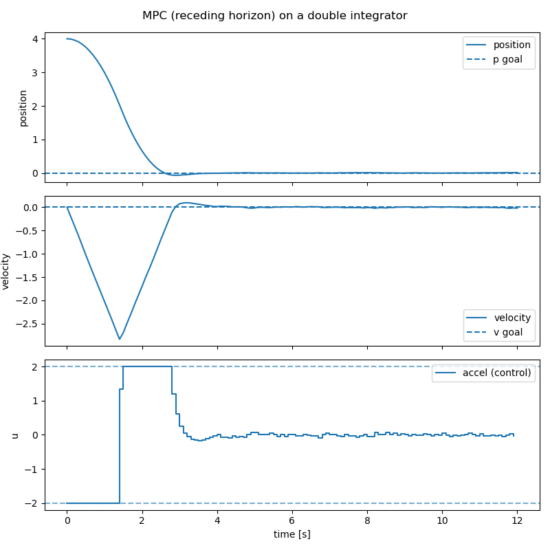
Figure 4.13: MPC for double integrator (small disturbance).
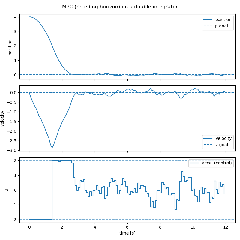
Figure 4.14: MPC for double integrator (large disturbance).
4.5 Model Predictive Path Integral Control
We have seen that numerical techniques–particularly gradient-based nonlinear programming methods–can be employed to solve trajectory optimization (TO) problems. Furthermore, solving TO problems repeatedly in an online fashion yields an implicit feedback policy, as in model predictive control (MPC).
The numerical methods discussed so far for TO rely on access to at least first-order derivatives of the objective and constraint functions. In this section, we introduce a different class of methods, known as model predictive path integral (MPPI) control (Williams et al. 2016). These methods do not require derivative information; instead, they rely solely on evaluating the objective and constraints through forward simulations of the system dynamics.
Problem Formulation. We consider a general nonlinear discrete-time dynamical system \[ x_{t+1} = f_t(x_t, u_t), \qquad t = 0,\dots, N-1, \] with state \(x_t \in \mathbb{R}^n\) and control \(u_t \in \mathbb{R}^m\). Given an initial condition \(x_0 = \hat x_0\) (known), the finite-horizon trajectory optimization problem is \[ \begin{aligned} \min_{\{x_t,u_t\}_{t=0}^{N-1}} \quad & \Phi(x_N) \;+\; \sum_{t=0}^{N-1} \ell_t(x_t, u_t) \\ \text{s.t.} \quad & x_{t+1} = f_t(x_t, u_t), \quad t=0,\dots,N-1, \\ & x_0 = \hat x_0 \;\; (\text{given}). \end{aligned} \] Here, \(\ell_t\) is the stage (running) cost and \(\Phi\) is the terminal cost. A dynamically feasible trajectory \(\{x_t,u_t\}_{t=0}^{N-1}\) satisfies the dynamics constraints for all \(t\).
High-Level Idea of MPPI. MPPI is a sampling-based, derivative-free, receding-horizon controller derived from path-integral / information-theoretic control. Instead of solving the constrained optimization problem via gradients or linearizations, MPPI:
Maintains a nominal open-loop control sequence \(U = \{u_0,\dots,u_{N-1}\}\).
At the current state \(x_0\), it samples many noisy control sequences \(u_t + \epsilon_t^{(k)}\) for rollouts \(k=1,\dots,K\).
For each rollout, it propagates the dynamics forward and scores the trajectory with the same task cost \(\Phi + \sum \ell_t\).
It soft-min aggregates the sampled control perturbations with weights \[ w_k \; \propto \; \exp\!\Big(-\tfrac{1}{\lambda}\big(S^{(k)} - \min_j S^{(j)}\big)\Big), \] where \(S^{(k)}\) is the total cost of the \(k\)-th trajectory and \(\lambda>0\) is a temperature parameter.
It updates the nominal sequence by adding the weighted average of the sampled perturbations: \[ u_t \;\leftarrow\; u_t \;+\; \sum_{k=1}^K \bar w_k\, \epsilon_t^{(k)}, \qquad \bar w_k = \frac{w_k}{\sum_j w_j}. \] Optionally, if computational budget permits, one can repeat steps 1 to 5 for multiple iterations. If the control actions need to satisfy hard bounds, we can project \(u_t\) to the feasible set.
It applies only the first control \(u_0\) to the real system, shifts the sequence forward, and repeats at the next time step (receding horizon).
Key properties.
Works with general nonlinear dynamics and arbitrary costs; no gradients, no linearization required.
Robustness arises from the soft-min over many trajectories.
Parallelizable (GPU-friendly) because rollouts are independent.
Computational details of the MPPI algorithm are given as follows.
Rollouts and total cost. Given current state \(x_0\) and nominal controls \(U=\{u_t\}_{t=0}^{N-1}\), draw \(K\) noise sequences \[ \epsilon^{(k)} = \{\epsilon_0^{(k)},\ldots,\epsilon_{N-1}^{(k)}\}, \qquad \epsilon_t^{(k)} \sim \mathcal{N}(0, \Sigma_t) \] (possibly time-correlated for smoothness). For each \(k \in [1,K]\):
- Simulate \[ \tilde u_t^{(k)} = u_t + \epsilon_t^{(k)}, \qquad x_{t+1}^{(k)} = f_t \big(x_t^{(k)}, \tilde u_t^{(k)}\big), \quad x_0^{(k)} = x_0. \]
- Accumulate the total trajectory cost \[ S^{(k)} \;=\; \Phi \big(x_N^{(k)}\big)\;+\; \sum_{t=0}^{N-1} \ell_t \big(x_t^{(k)}, \tilde u_t^{(k)}\big). \]
Exponential weights (soft-min). Stabilize by subtracting the minimum cost: \[ w_k \;=\; \exp\!\Big(-\tfrac{1}{\lambda}\big(S^{(k)} - S_{\min}\big)\Big), \quad S_{\min} := \min_j S^{(j)}. \] Normalize \(\bar w_k = w_k / \sum_j w_j\).
Control update. For each time \(t=0,\dots,N-1\), update \[ u_t \;\leftarrow\; u_t \;+\; \sum_{k=1}^K \bar w_k\, \epsilon_t^{(k)}. \] If control is bounded, project the controls onto the feasible sets.
Practical knobs.
\(K\): number of rollouts (compute–performance tradeoff).
\(\lambda\): temperature (smaller \(\Rightarrow\) greedier toward the best rollouts).
\(\Sigma_t\): exploration covariance; can use AR(1) temporal correlation for smooth controls.
Example 4.7 (MPPI for Pendulum Swing Up) We apply the MPPI controller, in an MPC receding-horizon control fashion to the pendulum swing-up problem.
We use \(K=16\) rollouts and set \(\lambda=1\).
When \(\Sigma_t\) is large enough, for example, when we set the standard deviation of the noise to be \(2\), the MPPI controller can successfully swing up the pendulum, demonstrating a highly sophisticated motion plan as shown in Fig. 4.15.
Figure 4.15: Pendulum swing-up using MPPI (large exploration).
However, when \(\Sigma_t\) is too small, when we set the standard deviation of the noise to be \(0.1\), the MPPI controller fails at the task, as shown in Fig. 4.16.
You can play with the code here.

Figure 4.16: Pendulum swing-up using MPPI (small exploration).
4.5.1 Information-Theoretic Derivation of MPPI
We now derive Model Predictive Path Integral (MPPI) control from an information-theoretic (KL-control / control-as-inference) viewpoint. We proceed from a variational free-energy objective to the Gibbs (Boltzmann) optimal trajectory law, then obtain the practical MPPI update via moment projection and importance sampling.
Let a finite-horizon trajectory be \(\tau=(x_0,u_0,\dots,u_{H-1},x_H)\) generated by discrete-time dynamics \[ x_{t+1} = f_t(x_t,u_t), \quad t=0,\dots,H-1. \] Let \(S(\tau)\) denote the total trajectory cost (e.g., terminal \(+\) running \(+\) control effort). Let \(p(\tau)\) be a baseline (prior) trajectory distribution (e.g., nominal/uncontrolled dynamics plus a prior over control sequences).
We seek a controlled trajectory distribution \(q(\tau)\) that trades performance against deviation from the prior via: \[ \mathcal{F}(q)\;=\;\mathbb{E}_{q}\big[S(\tau)\big]\;+\;\lambda\,\mathrm{KL} \big(q(\tau)\,\|\,p(\tau)\big),\qquad \lambda>0. \tag{4.97} \] This is convex in \(q\) (the first term is linear in \(q\) while the second term is convex in \(q\)). The scalar \(\lambda\) plays the role of a temperature (risk-sensitivity / exploration level).
Gibbs–Boltzmann Optimum. Our goal is now to minimize \(\mathcal{F}(q)\) over all normalized densities \(q(\tau)\). This is a constrained convex optimization in \(q\). Therefore, we can formulate the Lagrangian and derive the KKT optimality conditions.
Exercise 4.2 Formulate the Lagrangian for problem (4.97) and find its KKT optimality conditions.
Solving the KKT optimality conditions, one can find the optimal solution \[ q^\star(\tau)\ \propto\ p(\tau)\,\exp\!\big(-S(\tau)/\lambda\big). \] Thus, with proper normalization, we have \[ q^\star (\tau)\;=\;\frac{1}{Z}\;p(\tau)\,\exp\!\big(-S(\tau)/\lambda\big), \qquad Z \;=\; \int p(\tau)\,e^{-S(\tau)/\lambda}\,d\tau \;=\;\mathbb{E}_{p}\!\big[e^{-S/\lambda}\big]. \tag{4.98} \] Plugging \(q^\star\) back into \(\mathcal{F}\) gives the free-energy identity: \[ \min_{q}\Big\{\mathbb{E}_{q}[S]+\lambda\,\mathrm{KL}(q\|p)\Big\} \;=\; -\lambda \log \mathbb{E}_{p} \left[e^{-S/\lambda}\right]. \tag{4.99} \]
From Gibbs–Boltzmann Optimum to MPPI Updates. Let a trajectory be \(\tau=(x_0,u_0,\dots,u_{H-1},x_H)\) with dynamics \(x_{t+1}=f_t(x_t,u_t)\). We introduce a baseline (prior) trajectory distribution \(p(\tau)\) as the law induced by: \[ \mathbf v=(v_0,\dots,v_{H-1}) \sim \mathcal N(\mathbf U,\Sigma), \qquad v_t = u_t + \epsilon_t,\quad \epsilon_t\sim\mathcal N(0,\Sigma_t), \] and rolling out the dynamics with controls \(u_t=v_t\). Here \(\mathbf U = (u_0,\dots,u_{H-1})\) is the current nominal control sequence.
Given a trajectory cost \(S(\tau)\) and temperature \(\lambda>0\), the optimal controlled trajectory law is \[ q^\star(\tau)\;=\;\frac{1}{Z}\,p(\tau)\,\exp\!\big(-S(\tau)/\lambda\big), \qquad Z=\mathbb{E}_{p}\!\left[e^{-S/\lambda}\right]. \] Because of nonlinear dynamics and the exponential tilt by \(S\), \(q^\star\) is generally not Gaussian, even if \(p\) is.
MPPI approximates \(q^\star\) by maintaining a Gaussian over the control sequence with the same covariance \(\Sigma\) and a tunable mean \(\mathbf U=(u_0,\dots,u_{H-1})\): \[ \pi_{\mathbf U}(\mathbf v)\;=\;\mathcal N(\mathbf v;\mathbf U,\Sigma). \] MPPI projects \(q^\star\) onto this family by minimizing \(\mathrm{KL}\big(\pi_{\mathbf U}\,\|\,q^\star\big)\) while holding \(\Sigma\) fixed. For Gaussians with fixed covariance, this yields moment matching of the mean: \[ \mathbf U_{\text{new}} \;=\; \mathbb{E}_{q^\star}[\mathbf v]. \]
To perform this moment matching, we write \(v_t=u_t+\epsilon_t\). Then \[ u_{t,\text{new}} \;=\; \mathbb{E}_{q^\star}[v_t] = u_t + \mathbb{E}_{q^\star}[\epsilon_t]. \] We cannot sample \(q^\star\) directly, but by the Gibbs–Boltzmann form and importance sampling: \[ \mathbb{E}_{q^\star}[g(\tau)] = \frac{\mathbb{E}_{p}[\,g(\tau)\,e^{-S(\tau)/\lambda}\,]}{\mathbb{E}_{p}[\,e^{-S(\tau)/\lambda}\,]}. \] Choosing \(g(\tau)=\epsilon_t\) and using rollouts \(\{\tau^{(k)}\}_{k=1}^K\sim p\) with costs \(S^{(k)}\) and noises \(\epsilon_t^{(k)}\) gives the MPPI update: \[ \boxed{ u_t \;\leftarrow\; u_t \;+\; \sum_{k=1}^K \bar w_k\,\epsilon_t^{(k)}, \qquad \bar w_k = \frac{\exp\!\big(-\tfrac{1}{\lambda}(S^{(k)}-S_{\min})\big)} {\sum_j \exp\!\big(-\tfrac{1}{\lambda}(S^{(j)}-S_{\min})\big)}. } \] Here \(S_{\min}=\min_k S^{(k)}\) is a numerical stabilizer that cancels in the ratio.
Takeaway.
\(p(\tau)\): baseline trajectory law induced by Gaussian exploratory controls and the dynamics.
\(q^\star(\tau)\): Gibbs–Boltzmann tilt of \(p\), not Gaussian in general.
MPPI approximates \(q^\star\) by a Gaussian over controls with fixed covariance \(\Sigma\) and updates the mean by importance-weighted averaging of sampled noise, yielding the standard MPPI updates used in practice.
4.6 Rapidly Exploring Random Tree
In Section 4.5, we examined the effectiveness of one particular sampling-based planning method—MPPI—for solving trajectory-planning problems, noting that it is often less susceptible to local minima than nonlinear-programming-based approaches. More broadly, sampling-based motion planning encompasses a wide family of algorithms, extensive enough to merit an entire semester for a comprehensive treatment. For readers interested in exploring this area further, the textbooks (LaValle 2006) and (Choset et al. 2005) provide excellent overviews.
In this section, we introduce one of the most widely used sampling-based algorithms: the rapidly exploring random tree (RRT). We will begin with the case of kinematic motion planning, in which the system or robot is modeled as a point mass without dynamics, and then extend the discussion to kinodynamic motion planning, where the system’s dynamics must be taken into account.
4.6.1 Kinematic Motion Planning
Problem Setup. We consider a robot with configuration space \(\mathcal{C} \subset \mathbb{R}^d\). Obstacles occupy \(\mathcal{C}_\mathrm{obs}\), and the free space is \[ \mathcal{C}_\mathrm{free} = \mathcal{C} \setminus \mathcal{C}_\mathrm{obs}. \] Given a start configuration \(q_\mathrm{start} \in \mathcal{C}_\mathrm{free}\) and a goal region \(\mathcal{C}_\mathrm{goal} \subset \mathcal{C}_\mathrm{free}\), the objective is to find a collision-free path \[ \sigma : [0,1] \to \mathcal{C}_\mathrm{free}, \qquad \sigma(0) = q_\mathrm{start}, \ \sigma(1) \in \mathcal{C}_\mathrm{goal}. \] Here, \(\sigma(\cdot)\) is a continuous curve in the configuration space \(\mathcal{C}\) that connects the start position to the goal region. A path can be represented in several ways (e.g., piecewise-polynomial splines); in this section we adopt a piecewise-linear representation: the path is a sequence of waypoints \((q_0, q_1, \dots, q_M)\) joined by straight-line segments in \(\mathcal{C}\), i.e., \[ \sigma(s)= (1-s)\,q_i + s\,q_{i+1}, \quad s\in[0,1], \ \ i=0,\dots,M-1. \]
The RRT algorithm requires the following components.
Sampler. We require a mechanism to draw random configurations in free space. The simplest choice is uniform sampling: \[ q_{\mathrm{rand}} \sim \mathcal{U}\!\left(\mathcal{C}_{\mathrm{free}}\right), \] optionally with goal bias: introduce \(B \sim \mathrm{Bernoulli}(p_{\mathrm{goal}})\) and set \[ q_{\mathrm{rand}} = \begin{cases} \text{a sample from } \mathcal{C}_{\mathrm{goal}}, & \text{if } B=1,\\ \text{a sample from } \mathcal{C}_{\mathrm{free}}, & \text{if } B=0. \end{cases} \] To perform such sampling, we require that, given any configuration \(q \in \mathcal{C}\), we can check its membership in \(\mathcal{C}_{\mathrm{free}}\), \(\mathcal{C}_{\mathrm{obs}}\), and \(\mathcal{C}_{\mathrm{goal}}\).
Metric (Distance Function). We need a distance \(d:\mathcal{C}\times\mathcal{C}\to \mathbb{R}_{\ge 0}\) to compare configurations. Common choices: \[ d(q_i,q_j) = \|W(q_i-q_j)\|_2, \] where \(W\) is a positive-definite weighting (e.g., to account for different joint ranges).
For \(\text{SE}(2)\) or \(\text{SE}(3)\) manifolds,
- handle angular wrap-around (e.g., modulo \(2\pi\)),
- optionally combine translational and rotational parts with different weights,
- use a geodesic or a local chart; for rotations, a distance induced by the Lie group metric.
Sometimes \(d\) is defined in task space via forward kinematics \(x=\Phi(q)\) (here \(q\) represents the joint angles of a robot arm and \(\Phi(q)\) returns the position of the robot’s end-effector): \[ d(q_i,q_j)=\|\Phi(q_i)-\Phi(q_j)\|, \] useful when end-effector placement matters more than joint motion.
Nearest-Neighbor Query. Given the current tree \(T\) with vertex set \(V(T)\), select the closest existing node to the new sample: \[ q_{\mathrm{near}} \in \arg\min_{q\in V(T)} d\big(q,\,q_{\mathrm{rand}}\big). \]
Implementation notes.
- Use spatial indices (kd-trees, ball trees, cover trees) for sublinear searches.
- Approximate nearest neighbor methods often suffice and substantially accelerate growth in higher dimensions.
Steering / Step Map. Move from \(q_{\mathrm{near}}\) toward \(q_{\mathrm{rand}}\) by at most a step size \(\eta>0\). In Euclidean \(\mathcal{C}\), \[ \Delta = q_{\mathrm{rand}} - q_{\mathrm{near}}, \qquad q_{\mathrm{new}} = q_{\mathrm{near}} + \alpha\,\Delta,\quad \alpha = \min\!\left\{1,\ \frac{\eta}{\|\Delta\|_2}\right\}. \] On manifolds (e.g., \(SE(3)\)), interpolate along a feasible local geodesic; for rotations, use group operations (e.g., \(q_{\mathrm{new}} = q_{\mathrm{near}}\exp(\alpha\,\log(q_{\mathrm{near}}^{-1}q_{\mathrm{rand}}))\)).
Tuning \(\eta\).
- Smaller \(\eta\) improves collision fidelity and resolution in narrow passages but slows exploration.
- Larger \(\eta\) accelerates coverage but can skip through feasible corridors.
Collision Checking (Local Planner Validity). Validate the entire segment between \(q_{\mathrm{near}}\) and \(q_{\mathrm{new}}\): \[ \text{ensure } \sigma(s)\in \mathcal{C}_{\mathrm{free}} \ \ \forall s\in[0,1], \quad \sigma(s)=(1-s)q_{\mathrm{near}}+s q_{\mathrm{new}}. \]
Resolution and robustness.
- Use a discretization step \(\delta\) small enough relative to obstacle feature size and robot footprint.
- For articulated robots, perform swept-volume or continuous collision detection where possible; otherwise sample sufficiently along the edge (in joint and time parameter \(s\)).
- Inflate obstacles or deflate the robot model slightly to build clearance margins.
Stopping / Success Criteria. Let the goal be a set \(\mathcal{C}_{\mathrm{goal}}\) (e.g., a ball of radius \(\varepsilon\) around a target pose). Declare success when \[ q_{\mathrm{new}} \in \mathcal{C}_{\mathrm{goal}}. \]
Common termination rules.
- Maximum number of iterations or samples.
- Time budget exhausted (anytime behavior).
- Early stop after first solution (RRT) or continue to refine with rewiring (RRT*).
Post-processing (optional).
- Shortcutting: repeatedly replace subpaths by direct segments if collision-free.
- Smoothing: fit splines to waypoints while maintaining clearance, or re-optimize locally.
We are ready to present the RRT algorithm.
Algorithm: Rapidly-Exploring Random Tree (RRT) — Kinematic Case
Inputs: start configuration \(q_{\mathrm{start}} \in \mathcal{C}_{\mathrm{free}}\); goal region \(\mathcal{C}_{\mathrm{goal}} \subset \mathcal{C}_{\mathrm{free}}\); step size \(\eta>0\); goal-bias \(p_{\mathrm{goal}} \in [0,1]\); iteration budget \(N\); metric \(d:\mathcal{C}\times\mathcal{C}\to\mathbb{R}_{\ge 0}\); collision checker for segments in \(\mathcal{C}\); nearest-neighbor data structure over the current vertex set.
Initialize the tree \(T\) with vertex set \(V(T)\gets\{q_{\mathrm{start}}\}\) and no edges.
For \(i=0,1,2,\dots,N-1\)
Goal-biased sampling. Draw \(B\sim\mathrm{Bernoulli}(p_{\mathrm{goal}})\) and set \[ q_{\mathrm{rand}} \sim \begin{cases} \mathcal{U}(\mathcal{C}_{\mathrm{goal}}), & \text{if } B=1,\\[2pt] \mathcal{U}(\mathcal{C}_{\mathrm{free}}), & \text{if } B=0. \end{cases} \]
Nearest neighbor. Select \[ q_{\mathrm{near}} \in \arg\min_{q\in V(T)} d\!\left(q,\,q_{\mathrm{rand}}\right). \]
Steering (bounded step). Let \(\Delta := q_{\mathrm{rand}}-q_{\mathrm{near}}\) in a local chart of \(\mathcal{C}\) (with appropriate handling of angles/manifold coordinates). Define \[ \alpha := \min\!\left\{1,\ \frac{\eta}{\|\Delta\|}\right\},\qquad q_{\mathrm{new}} := q_{\mathrm{near}} + \alpha\,\Delta. \] (On manifolds, replace the affine step with interpolation along a local geodesic.)
Collision checking. Verify the straight segment \[ \sigma(s) = (1-s)\,q_{\mathrm{near}} + s\,q_{\mathrm{new}},\quad s\in[0,1], \] satisfies \(\sigma(s)\in\mathcal{C}_{\mathrm{free}}\) for all sampled \(s\) (or via continuous collision detection).
Tree update. If the segment is collision-free, append the vertex and edge: \[ V(T)\gets V(T)\cup\{q_{\mathrm{new}}\},\qquad E(T)\gets E(T)\cup\{(q_{\mathrm{near}}\rightarrow q_{\mathrm{new}})\}. \]
Success test. If \(q_{\mathrm{new}}\in \mathcal{C}_{\mathrm{goal}}\), terminate and return the path formed by the unique tree route from \(q_{\mathrm{start}}\) to \(q_{\mathrm{new}}\).
Stopping: If no success after \(N\) iterations (or upon time-budget exhaustion), return failure (or the best partial progress if maintained).
Properties.
Probabilistic completeness: If a solution exists, the probability that RRT finds one approaches 1 as \(N \to \infty\).
Not optimal: The first-found solution can be far from shortest; RRT does not asymptotically improve path quality.
4.6.1.1 Make RRT Optimal: RRT*
The classical RRT is probabilistically complete but not optimal. To obtain asymptotic optimality (i.e., the best-path cost converges to the global optimum as the number of samples \(N\to\infty\)), we use RRT*: a cost-aware variant that (i) selects parents by minimizing cost-to-come and (ii) rewires nearby nodes to improve their costs when possible.
Key Ideas Behind RRT*:
Cost functional. Let \(c(\cdot)\) denote path cost (e.g., length or any additive, nonnegative, Lipschitz continuous cost). For an edge between two configurations \(q\) and \(q'\), write \(c(q\to q')\) and define \[ c(q') \;=\; \min_{(q \to q') \in E(T)} \big\{c(q) + c(q\to q')\big\}, \] where \(E(T)\) is the set of tree edges.
Near set. Rather than connecting to only the nearest node, examine a ball of neighbors around the new sample \(q_{\mathrm{new}}\) whose radius shrinks with \(n\): \[ r_n \;=\; \gamma \left(\frac{\log n}{n}\right)^{1/d}, \] where \(d\) is the dimension of \(\mathcal{C}\) and \(\gamma>\gamma^\ast\) is a constant depending on the measure of \(\mathcal{C}_{\mathrm{free}}\). (Alternative: \(k\)-nearest with \(k_n \ge k_0 \log n\).)
Choose parent by cost. Among the near nodes that can connect to \(q_{\mathrm{new}}\) collision-free, pick the parent that minimizes total cost-to-come.
Rewire. Attempt to improve each neighbor \(q\) by re-connecting it through \(q_{\mathrm{new}}\) if this reduces \(c(q)\) while preserving feasibility.
Asymptotic optimality. Under standard assumptions (e.g., \(\delta\)-robustly feasible problem, absolutely continuous sampling over \(\mathcal{C}_{\mathrm{free}}\), consistent local planner, and the \(r_n\) or \(k_n\) schedules above), the best path cost in the tree converges almost surely to the global optimum.
The RRT* Algorithm is presented below.
Algorithm: RRT* (Asymptotically Optimal RRT)
Inputs: \(q_{\mathrm{start}}\in\mathcal{C}_{\mathrm{free}}\), goal region \(\mathcal{C}_{\mathrm{goal}}\subset\mathcal{C}_{\mathrm{free}}\); metric \(d\); step size \(\eta>0\); goal-bias \(p_{\mathrm{goal}}\in[0,1]\); iteration budget \(N\); neighbor schedule \(r_n=\gamma(\tfrac{\log n}{n})^{1/d}\) (or \(k_n\ge k_0\log n\)).
Initialize \(T\) with \(V(T)\gets\{q_{\mathrm{start}}\}\), \(E(T)\gets\emptyset\), \(c(q_{\mathrm{start}})=0\).
For \(i=0,1,2,\dots,N-1\)
Goal-biased sampling. Draw \(B\sim\mathrm{Bernoulli}(p_{\mathrm{goal}})\) and set \[ q_{\mathrm{rand}} \sim \begin{cases} \mathcal{U}(\mathcal{C}_{\mathrm{goal}}), & B=1,\\ \mathcal{U}(\mathcal{C}_{\mathrm{free}}), & B=0. \end{cases} \]
Nearest and steer. Choose \[ q_{\mathrm{near}}\in\arg\min_{q\in V(T)} d\big(q,\,q_{\mathrm{rand}}\big),\quad q_{\mathrm{new}} := q_{\mathrm{near}} + \alpha\big(q_{\mathrm{rand}}-q_{\mathrm{near}}\big), \] with \(\alpha=\min\{1,\eta/\|q_{\mathrm{rand}}-q_{\mathrm{near}}\|\}\). If the segment \([q_{\mathrm{near}},q_{\mathrm{new}}]\) is not collision-free, continue.
Near set. Denote \(n = |V(T)|\) as the number of nodes in the current tree, let \[ \mathcal{N}_n(q_{\mathrm{new}}) \;=\; \big\{q\in V(T): d(q,q_{\mathrm{new}})\le r_n\big\}. \]
Choose parent by cost. Set provisional parent \(\bar{q}\gets q_{\mathrm{near}}\) with provisional cost \[ \bar{c} \;=\; c(q_{\mathrm{near}}) + c\!\left(q_{\mathrm{near}}\to q_{\mathrm{new}}\right). \] For each \(q\in \mathcal{N}_n(q_{\mathrm{new}})\) such that the segment \([q,q_{\mathrm{new}}]\) is collision-free, if \[ c(q) + c(q\to q_{\mathrm{new}}) < \bar{c}, \] then update \(\bar{q}\gets q\), \(\bar{c}\gets c(q)+c(q\to q_{\mathrm{new}})\).
Insert. Add \(q_{\mathrm{new}}\) to \(V(T)\), add edge \((\bar{q}\rightarrow q_{\mathrm{new}})\) to \(E(T)\), and set \(c(q_{\mathrm{new}})\gets \bar{c}\).
Rewire. For each \(q\in\mathcal{N}_n(q_{\mathrm{new}})\) such that segment \([q_{\mathrm{new}},q]\) is collision-free, if \[ c(q_{\mathrm{new}}) + c(q_{\mathrm{new}}\to q) < c(q), \] then change \(q\)’s parent to \(q_{\mathrm{new}}\) and update \(c(q)\) (and, if maintained, the costs of its descendants).
Goal check. If \(q_{\mathrm{new}}\in\mathcal{C}_{\mathrm{goal}}\), record/update the current best path.
Stopping: Terminate upon time/iteration budget; return the best path found (its cost decreases and converges to the optimal value almost surely).
Intuition of why RRT* is optimal:
The shrinking neighbor radius \(r_n\propto(\log n/n)^{1/d}\) ensures that, as \(n\) grows, the graph locally approximates the geometry of \(\mathcal{C}_{\mathrm{free}}\) with just enough connectivity to avoid fragmentation.
Parent selection and rewiring implement dynamic programming over this increasingly dense graph, continually lowering costs.
Under regularity and \(\delta\)-clearance, any optimal path can be covered by a sequence of balls of radius \(r_n\); with high probability the tree includes nodes in each ball, enabling a piecewise improvement that converges to the optimal path cost.
Common Enhancements (Keep Optimality, Speed It Up):
- Informed RRT*: after the first solution of cost \(C^\star\), sample within the informed subset that can still achieve cost \(<C^\star\).
- Batch variants (BIT*): combine sampling with incremental graph search for faster convergence.
- Pruning: discard nodes whose best possible heuristic cannot beat the current best cost.
Example 4.8 (RRT* for 2D Kinematic Motion Planning) We can apply RRT* to find collision-free paths from a start position to a goal region.
You can play with the code here.
The code provides an implementation of RRT* from scratch. For an off-the-shelf implementation of RRT* and other motion planning algorithms, we recommend the Open Motion Planning Library (OMPL).
Figure 4.17: RRT* finding collision-free paths.
4.6.2 Kinodynamic Motion Planning
Problem Setup. Let the state space be \(\mathcal{X}\subset\mathbb{R}^{d}\) and the control space be \(\mathcal{U}\subset\mathbb{R}^{m}\). The robot obeys differential constraints \[ \dot{x}(t)=f\big(x(t),u(t)\big), \qquad u(t)\in\mathcal{U}, \] with \(f\) locally Lipschitz in \(x\) and measurable in \(u\). Obstacles occupy \(\mathcal{X}_\mathrm{obs}\subset\mathcal{X}\); the free space is \[ \mathcal{X}_\mathrm{free}=\mathcal{X}\setminus \mathcal{X}_\mathrm{obs}. \] Given \(x_\mathrm{start}\in\mathcal{X}_\mathrm{free}\) and a goal region \(\mathcal{X}_\mathrm{goal}\subset\mathcal{X}_\mathrm{free}\), we seek a feasible trajectory \[ x:[0,T]\to\mathcal{X}_\mathrm{free},\quad u:[0,T]\to\mathcal{U},\quad \dot{x}=f(x,u),\ x(0)=x_\mathrm{start},\ x(T)\in\mathcal{X}_\mathrm{goal}. \] For optimal kinodynamic planning, we seek to minimize the additive cost \[ J[x,u] \;=\; \phi\big(x(T)\big) \;+\; \int_{0}^{T} \ell\big(x(t),u(t)\big)\,dt, \] e.g., minimum time (\(\ell\equiv 1\)), energy, or path-length surrogates.
As in the kinematic case, we grow a tree—now in state space—whose edges are dynamically feasible rollouts.
The RRT* algorithm for kinodynamic planning requires the following components.
State sampler. Draw states in free space with optional goal bias: \[ x_{\mathrm{rand}} \sim \text{Uniform}\big(\mathcal{X}_{\mathrm{goal}}\big)\ \text{w.p. }p_\mathrm{goal},\quad x_{\mathrm{rand}} \sim \text{Uniform} \big(\mathcal{X}_{\mathrm{free}}\big)\ \text{otherwise}. \] Must support membership tests \(x\in\mathcal{X}_\mathrm{free}\) and \(x\in\mathcal{X}_\mathrm{goal}\).
Metric / heuristic. A distance \(d:\mathcal{X}\times\mathcal{X}\to\mathbb{R}_{\ge 0}\) guides nearest-neighbor queries and “move-toward” decisions.
- Weighted Euclidean in a local chart (with angle wrap-around) is common: \[ d(x_i,x_j)=\|W(x_i-x_j)\|_2. \]
- Prefer system-aware local distances when available (e.g., Dubins/Reeds–Shepp, double integrator, LQR).
Example 4.9 (Distance Metric for Dubins Car) In kinodynamic planning, two states that are close in Euclidean norm can still be far in terms of actual time/effort to move between them under the robot’s dynamics. A system-aware local distance replaces a geometric norm \[ \|x_i-x_j\| \] with a control distance \[ d_f(x_i,x_j)\ :=\ \inf_{u(\cdot),\,T}\;\Big\{ \int_0^T \ell\big(x(t),u(t)\big)\,dt\ \Big|\ \dot x=f(x,u),\ x(0)=x_i,\ x(T)=x_j \Big\}, \] i.e., the optimal local connection cost (time, path length, energy) for your specific system \(f\). This distance respects:
- Nonholonomy (e.g., car cannot sidestep).
- Bounds (e.g., max turn rate, min turning radius, velocity limits).
- Asymmetry (forward-only systems: going from \(x_i\) to \(x_j\) may cost more than reverse).
In practice we use closed-form local connectors when they exist or fast approximations (e.g., LQR quadratic form near an operating point). When nothing closed-form exists, we keep Euclidean for indexing but score candidates with a rollout-based cost.
For example, we consider the Dubins car system.
Model & constraints.
- State \(q=(x,y,\theta)\in \mathbb{R}^2\times \mathbb{S}^1\).
- Controls: constant forward speed \(v>0\); turn rate \(\omega\) with \(|\omega|\le \omega_{\max}\).
- Min turning radius \(R = v/\omega_{\max}\).
- Kinematics: \[ \dot x = v\cos\theta,\quad \dot y = v\sin\theta,\quad \dot\theta = \omega,\quad |\omega|\le \omega_{\max},\quad v\ge 0. \]
- No reverse gear (nonnegative speed).
Shortest feasible paths. Between two poses \(q_s,q_g\) (with no obstacles), the shortest path with curvature bound \(1/R\) is a sequence of at most three primitives:
- C: constant-curvature arc (left \(L\) or right \(R\)) of radius \(R\),
- S: straight segment.
Only six word types can be optimal:
\[
\mathcal{W} = \{ \mathbf{LSL}, \mathbf{RSR}, \mathbf{LSR}, \mathbf{RSL}, \mathbf{RLR}, \mathbf{LRL} \}.
\]
Normalization. Translate/rotate so \(q_s\) is at the origin with heading \(0\). Scale coordinates by \(R\) (so the min radius becomes 1). Let the normalized goal be \((\bar{x},\bar{y},\bar{\theta})\).
Closed-form lengths. Each word has analytic formulas for the three segment lengths \((t,p,q)\) (two arc angles and a straight length) derived from the circle tangency geometry; e.g., for LSL: \[ \begin{aligned} \text{Let }&d=\sqrt{\bar{x}^2+\bar{y}^2},\ \phi=\mathrm{atan2}(\bar{y},\bar{x}),\\ t&=\mathrm{mod}_{2\pi}\big(-\phi\big),\\ p&=\sqrt{\max(0,\,d^2-2+2\cos(\bar{\theta}-\phi))}\ \ \text{(straight length)},\\ q&=\mathrm{mod}_{2\pi}\big(\bar{\theta}-\phi\big), \end{aligned} \]
The Dubins length is the minimum total length over all valid words: \[ L_\text{Dubins}(q_s,q_g) \;=\; R\,\min_{\text{word}\in\mathcal{W}}\ \big(t+p+q\big), \] and with constant \(v\), minimum time is \(T_\text{Dubins}=L_\text{Dubins}/v\).
The Reeds–Shepp car model extends the Dubins car model to allow reverse gear.
Nearest neighbor. Given vertices \(V(T)\subset\mathcal{X}\), \[ x_{\mathrm{near}} \in \arg\min_{x\in V(T)} d\big(x,\,x_{\mathrm{rand}}\big). \] Use kd/ball trees or Approximate Nearest Neighbor (ANN) structures in a consistent local chart.
Forward “steering” (local planner). When no closed-form two-point connector exists, forward propagate from \(x_{\mathrm{near}}\) by sampling controls and durations and integrating: \[ u \sim \mathcal{D}_u,\ \ \tau\sim\mathcal{D}_\tau,\ \ x^+(t) = \Phi \big(x_{\mathrm{near}},u,t\big),\ t\in[0,\tau], \] where \(\Phi\) is the numerical flow (e.g., RK4 with step \(h\)). Here \(\mathcal{D}_u\) is the probability distribution over controls used to sample a candidate open-loop input (e.g., uniform over a bounded box, Gaussian around a heuristic, a discrete set of motion primitives, or biased by a policy); and \(\mathcal{D}_\tau\) is the distribution over rollout durations (e.g., uniform on \([0,\tau_{\max}]\), a fixed shortlist of durations, or a geometric/exponential prior favoring short motions). Keep a rollout only if the entire trajectory stays in \(\mathcal{X}_\mathrm{free}\). The edge cost is \[ c\!\left(x_{\mathrm{near}}\!\to\!x_{\mathrm{new}}\right)=\int_{0}^{\tau}\ell\big(x^+(t),u\big)\,dt. \] If a steering function exists for your system (e.g., Dubins, LQR-QR), use it in place of random propagation.
Collision checking (trajectory validity). Validate the continuous rollout (time-discretized sufficiently for geometry and dynamics).
Neighbor set for rewiring. With \(n=|V(T)|\), use the RRT* radius schedule in state dimension \(d\): \[ r_n=\gamma \Big(\tfrac{\log n}{n}\Big)^{1/d} \quad\text{or}\quad k\text{-nearest with }k_n \ge k_0 \log n. \] Only neighbors reachable by a feasible local planner are considered connectable.
Costs. Each node stores cost-to-come \(c(x)\) (integral of \(\ell\) along the tree path). Parent selection and rewiring compare integrated edge costs from actual feasible rollouts (or optimal local connectors).
Stopping / success. Success when a node lies in \(\mathcal{X}_\mathrm{goal}\). As an anytime method, continue to improve cost by rewiring until time/iteration budget is exhausted.
The following pseudocode presents RRT* for kinodynamic motion planning.
Algorithm: RRT* — Kinodynamic Case
Inputs: initial state \(x_{\mathrm{start}}\in\mathcal{X}_\mathrm{free}\); goal region \(\mathcal{X}_\mathrm{goal}\subset\mathcal{X}_\mathrm{free}\); dynamics \(f\); metric \(d\); running cost \(\ell\), terminal cost \(\phi\); goal-bias \(p_{\mathrm{goal}}\in[0,1]\); budget \(N\); neighbor schedule \(r_n=\gamma(\tfrac{\log n}{n})^{1/d}\) (or \(k_n\ge k_0\log n\)); forward-propagation integrator and control/duration samplers (or a system-specific steering method).
Initialize \(T\): \(V(T)\gets\{x_{\mathrm{start}}\}\), \(E(T)\gets\emptyset\), \(c(x_{\mathrm{start}})=0\).
For \(i=0,1,2,\dots,N-1\)
Goal-biased sampling. Draw \(x_{\mathrm{rand}}\) from \(\mathcal{X}_\mathrm{goal}\) with probability \(p_{\mathrm{goal}}\), else from \(\mathcal{X}_\mathrm{free}\).
Nearest. Select \(x_{\mathrm{near}}\in\arg\min_{x\in V(T)} d(x,\,x_{\mathrm{rand}})\).
Forward “steer”. Generate a batch \(\{(u_k,\tau_k)\}_{k=1}^{K}\), integrate \(\dot{x}=f(x,u_k)\) from \(x_{\mathrm{near}}\) up to \(\tau_k\), discard infeasible rollouts, and pick a candidate terminal \(x_{\mathrm{new}}\) (e.g., closest to \(x_{\mathrm{rand}}\) or lowest edge cost). If none feasible, continue.
Near set. With \(n=|V(T)|\), \[ \mathcal{N}_n(x_{\mathrm{new}})=\{x\in V(T): d(x,x_{\mathrm{new}})\le r_n\}. \]
Choose parent by cost (feasible-only). Provisional parent \(\bar{x}\gets x_{\mathrm{near}}\) with provisional cost \[ \bar{c}=c(x_{\mathrm{near}})+c\big(x_{\mathrm{near}}\!\to\!x_{\mathrm{new}}\big). \] For each \(x\in\mathcal{N}_n(x_{\mathrm{new}})\), attempt a feasible local connection \(x\to x_{\mathrm{new}}\). If feasible and \[ c(x) + c\big(x\!\to\!x_{\mathrm{new}}\big) < \bar{c}, \] set \(\bar{x}\gets x\) and \(\bar{c}\) accordingly.
Insert. Add \(x_{\mathrm{new}}\) to \(V(T)\); add edge \((\bar{x}\to x_{\mathrm{new}})\) (storing its control/duration); set \(c(x_{\mathrm{new}})=\bar{c}\).
Rewire (forward-only). For each \(x\in\mathcal{N}_n(x_{\mathrm{new}})\), attempt a feasible connection \(x_{\mathrm{new}}\to x\). If \[ c(x_{\mathrm{new}}) + c\big(x_{\mathrm{new}}\!\to\!x\big) < c(x), \] then change \(x\)’s parent to \(x_{\mathrm{new}}\) and update costs (and, if maintained, descendants).
Goal check. If \(x_{\mathrm{new}}\in\mathcal{X}_\mathrm{goal}\), record/update the current best trajectory.
Stopping: On budget exhaustion, return the best feasible trajectory \((x(\cdot),u(\cdot))\) found.
Practical Notes.
Local planner. Replace random forward propagation with analytic/local-optimal connectors when available (Dubins/Reeds–Shepp, LQR for linearized systems, double integrator), which dramatically accelerates convergence.
Hyperparameters. Batch size \(K\), duration bounds \(\tau_{\max}\), and integrator step \(h\) balance exploration vs. fidelity; smaller \(h\) and moderate \(\tau\) help in tight dynamics/geometry.
Heuristics. Informed sampling (admissible lower bounds on remaining cost), pruning by lower-bound estimates, and \(k\)-nearest neighborhoods can maintain optimality while improving speed.
Asymptotic Optimality. Under standard assumptions—\(\delta\)-robust feasibility, absolutely continuous sampling over \(\mathcal{X}_\mathrm{free}\), locally Lipschitz dynamics, nonnegative Lipschitz running cost, and a consistent local planner (feasible connections that approximate short motions)—the best trajectory cost produced by kinodynamic RRT* converges almost surely to the global optimum as \(N\to\infty\). Intuitively, the shrinking neighborhood \(r_n\propto(\log n/n)^{1/d}\) yields a graph that becomes dense in the reachable set, and parent selection plus rewiring implement dynamic programming over this increasingly rich local-connectivity structure.
Common Enhancements (keep optimality).
Informed RRT* with kinodynamic admissible heuristics (e.g., minimum-time or minimum-energy lower bounds).
Batch planners (e.g., BIT*) that merge sampling and search with system-aware heuristics.
Reachability and cost-based pruning to focus computation where improvements are still possible.
Example 4.10 (RRT* for Dubins Car) Continuning Example 4.9, we apply RRT* to collision-free kinodynamic path planning for the Dubins car model.
Fig. 4.18 shows the RRT* algorithm’s running process.
You can play with the code here.
A similar YouTube demonstration video can be found here.
Figure 4.18: RRT* for Dubins Car.