Chapter 2 Value-based Reinforcement Learning

In Chapter 1, we introduced algorithms for policy evaluation, policy improvement, and computing optimal policies in the tabular setting when the model is known. These dynamic-programming methods are grounded in Bellman consistency and optimality and come with strong convergence guarantees.

A key limitation of the methods in Chapter 1 is that they require the transition dynamics \(P(s' \mid s, a)\) to be known. While in some applications modeling the dynamics is feasible (e.g., the inverted pendulum), in many others it is costly or impractical to obtain an accurate model of the environment (e.g., a humanoid robot interacting with everyday objects).

This motivates relaxing the known-dynamics assumption and asking whether we can design algorithms that learn purely from interaction—i.e., by collecting data through environment interaction. This brings us to model-free reinforcement learning.

In this chapter we focus on value-based RL methods. The central idea is to learn the value functions—\(V(s)\) and \(Q(s,a)\)—from interaction with the environment and then leverage these estimates to derive (approximately) optimal policies. We begin with tabular methods and then move to function-approximation approaches (e.g., neural networks) for problems where a tabular representation is intractable.

2.1 Tabular Methods

Consider an infinite-horizon Markov decision process (MDP)
\[ \mathcal{M} = (\mathcal{S}, \mathcal{A}, P, R, \gamma), \] with a discount factor \(\gamma \in [0,1)\). We focus on the tabular setting where both the state space \(\mathcal{S}\) and the action space \(\mathcal{A}\) are finite, with cardinalities \(|\mathcal{S}|\) and \(|\mathcal{A}|\), respectively.

A policy is a stationary stochastic mapping
\[ \pi: \mathcal{S} \to \Delta(\mathcal{A}), \] where \(\pi(a \mid s)\) denotes the probability of selecting action \(a\) in state \(s\).

Unlike in Chapter 1, here we do not assume knowledge of the transition dynamics \(P\) or the reward function \(R\) (other than that \(R\) is deterministic). Instead, we assume we can interact with the environment and obtain trajectories of the form
\[ \tau = (s_0, a_0, r_0, s_1, a_1, r_1, \dots), \] by following a policy \(\pi\).

2.1.1 Policy Evaluation

We first consider the problem of estimating the value function of a given policy \(\pi\). Recall the definition of the state-value function associated with \(\pi\) is: \[\begin{equation} V^{\pi}(s) = \mathbb{E}\left[ \sum_{t=0}^{\infty} \gamma^t R(s_t, a_t) \mid s_0 = s \right], \tag{2.1} \end{equation}\] where the expectation is taken over the randomness of both the policy \(\pi\) and the transition dynamics \(P\).

2.1.1.1 Monte Carlo Estimation

The basic idea of Monte Carlo (MC) estimation is to approximate the value function \(V^\pi\) by averaging empirical returns observed from sampled trajectories generated under policy \(\pi\). Since the return is defined as the discounted sum of future rewards, MC methods replace the expectation in the definition of \(V^\pi\) with an average over sampled trajectories.

Episodic Assumption. To make Monte Carlo methods well-defined, we restrict attention to the episodic setup, where each trajectory terminates upon reaching a terminal state (and the rewards thereafter are always zero). This ensures that the return is finite and can be computed exactly for each trajectory. Concretely, if an episode terminates at time \(T\), the return starting from time \(t\) is \[\begin{equation} g_t = \sum_{k=0}^{T-t-1} \gamma^k r_{t+k} = r_t + \gamma r_{t+1} + \gamma^2 r_{t+2} + \dots + \gamma^{T-t-1} r_{T-1}. \tag{2.2} \end{equation}\]

Algorithmic Form. Let \(\mathcal{D}(s)\) denote the set of all time indices at which state \(s\) is visited across sampled episodes. Then the Monte Carlo estimate of the value function is \[\begin{equation} \hat{V}(s) = \frac{1}{|\mathcal{D}(s)|} \sum_{t \in \mathcal{D}(s)} g_t. \tag{2.3} \end{equation}\]

There are two common variants:

• First-visit MC: use only the first occurrence of \(s\) in each episode.
  
• Every-visit MC: use all occurrences of \(s\) within an episode.

Both variants converge to the same value function in the limit of infinitely many episodes.

Incremental Implementation. Monte Carlo can be written as an incremental stochastic-approximation update that uses the return \(g_t\) as the target and a diminishing step size. Let \(N(s)\) be the number of (first- or every-) visits to state \(s\) that have been used to update \(\hat V(s)\) so far, and let \(g_t\) be the return computed at a particular visit time \(t\in\mathcal{D}(s)\). Then the MC update is \[\begin{equation} \hat V(s) \;\leftarrow\; \hat V(s) + \alpha_{N(s)}\,\big( g_t - \hat V(s) \big), \qquad \alpha_{N(s)} > 0 \text{ diminishing.} \tag{2.4} \end{equation}\] A canonical choice is the sample-average step size \(\alpha_{N(s)} = 1/N(s)\), which yields the recurrence \[\begin{align} \hat V_{N}(s) = \hat V_{N-1}(s) + \tfrac{1}{N}\big(g_t - \hat V_{N-1}(s)\big) & = \Big(1-\tfrac{1}{N}\Big)\hat V_{N-1}(s) + \tfrac{1}{N}\, g_t \\ & = \frac{N-1}{N} \frac{1}{N-1} \sum_{i=1}^{N-1} g_{t,i} + \frac{1}{N} g_t \\ & = \frac{1}{N} \sum_{i=1}^N g_{t,i} \end{align}\] so that \(\hat V_{N}(s)\) equals the average of the \(N\) observed returns for \(s\) (i.e., Eq. (2.3)). In the above equation, I have used \(g_{t,i}\) to denote the \(i\)-th return before \(g_t\) was collected (and \(g_t = g_{t,N}\)). More generally, any diminishing schedule satisfying \[ \sum_{n=1}^\infty \alpha_n = \infty, \qquad \sum_{n=1}^\infty \alpha_n^2 < \infty \] (e.g., \(\alpha_n = c/(n+t_0)^p\) with \(1/2 < p \le 1\)) also ensures consistency in the tabular setting. In first-visit MC, \(N(s)\) increases by one per episode at most; in every-visit MC, \(N(s)\) increases at each occurrence of \(s\) within an episode.

Theoretical Guarantees.

1. Unbiasedness: For any state \(s\), the return \(g_t\) is an unbiased sample of \(V^\pi(s)\).
   \[ \mathbb{E}[g_t \mid s_t = s] = V^\pi(s). \]
2. Consistency: By the law of large numbers, as the number of episodes grows, \[ \hat{V}(s) \xrightarrow{\text{a.s.}} V^\pi(s). \]
3. Asymptotic Normality: The MC estimator converges at rate \(O(1/\sqrt{N})\), where \(N\) is the number of episodes used for the estimation.

Limitations. Despite its conceptual simplicity, MC estimation suffers from several drawbacks:

• It requires episodes to terminate, making it unsuitable for continuing tasks without artificial truncation.

• It can only update value estimates after an episode ends, which is data-inefficient.

• While unbiased, MC estimates often have high variance, leading to slow convergence.

These limitations motivate the study of Temporal-Difference (TD) learning, which updates value estimates online and can handle continuing tasks.

2.1.1.2 Temporal-Difference Learning

While Monte Carlo methods estimate value functions by averaging full returns from complete episodes, Temporal-Difference (TD) learning provides an alternative approach that updates value estimates incrementally after each step of interaction with the environment. The key idea is to combine the sampling of Monte Carlo with the bootstrapping of dynamic programming.

High-Level Intuition. TD learning avoids waiting until the end of an episode by using the Bellman consistency equation as a basis for updates. Recall that for any policy \(\pi\), the Bellman consistency equation reads: \[\begin{equation} V^\pi(s) = \mathbb{E}_{a \sim \pi(\cdot \mid s)} \left[ R(s,a) + \gamma \mathbb{E}_{s' \sim P(s' \mid s, a)} V(s') \right]. \tag{2.5} \end{equation}\] At a high level, TD learning turns the expectation in Bellman equation into sampling. At each step, it updates the current estimate of the value function toward a one-step bootstrap target: the immediate reward plus the discounted value of the next state. This makes TD methods more data-efficient and applicable to continuing tasks without terminal states.

Algorithmic Form. Suppose the agent is in state \(s_t\), takes action \(a_t \sim \pi(\cdot \mid s_t)\), receives reward \(r_t\), and transitions to \(s_{t+1}\). The TD(0) update rule is \[\begin{equation} \hat{V}(s_t) \;\leftarrow\; \hat{V}(s_t) + \alpha \big[ r_t + \gamma \hat{V}(s_{t+1}) - \hat{V}(s_t) \big], \tag{2.6} \end{equation}\] where \(\alpha \in (0,1]\) is the learning rate.

The term inside the brackets, \[\begin{equation} \delta_t = r_t + \gamma \hat{V}(s_{t+1}) - \hat{V}(s_t), \tag{2.7} \end{equation}\] is called the TD error. It measures the discrepancy between the current value estimate and the bootstrap target. The algorithm updates \(\hat{V}(s_t)\) in the direction of reducing this error.

Theoretical Guarantees.

1. Convergence in the Tabular Case: If each state is visited infinitely often and the learning rate sequence satisfies \[ \sum_t \alpha_t = \infty, \; \sum_t \alpha_t^2 < \infty \] then TD(0) converges almost surely to the true value function \(V^\pi\). For example, choosing \(\alpha_t = 1/(t+1)\) satisfies this condition. Section 2.1.2 provides a detailed proof of the convergence of TD learning.

2. Bias–Variance Tradeoff:

   • The TD target uses the current estimate \(\hat{V}(s_{t+1})\) rather than the true value, which introduces bias.

   • However, it has significantly lower variance than Monte Carlo estimates, often leading to faster convergence in practice.

   To see this, note that for TD(0), the target is a one-step bootstrap: \[ y_t = r_t + \gamma \hat{V}(s_{t+1}). \] This replaces the true value \(V^\pi(s_{t+1})\) with the current estimate \(\hat{V}(s_{t+1})\). As a result, \(y_t\) is biased relative to the true return. However, since it depends only on the immediate reward and the next state, the variance of \(y_t\) is much lower than that of the Monte Carlo target.

Limitations.

• TD(0) relies on bootstrapping, which introduces bias relative to Monte Carlo methods.

• Convergence can be slow if the learning rate is not chosen carefully.

In summary, Temporal-Difference learning addresses the major limitations of Monte Carlo estimation: it works in continuing tasks, updates online at each step, and is generally more sample-efficient. However, it trades away unbiasedness for bias–variance efficiency, motivating further extensions such as multi-step TD and TD(\(\lambda\)).

2.1.1.3 Multi-Step TD Learning

Monte Carlo methods use the full return \(g_t\), while TD(0) uses a one-step bootstrap. Multi-step TD learning generalizes these two extremes by using \(n\)-step returns as targets. In this way, multi-step TD interpolates between Monte Carlo and TD(0).

High-Level Intuition. The motivation is to balance the high variance of Monte Carlo with the bias of TD(0). Instead of waiting for a full return (MC) or using only one step of bootstrapping (TD(0)), multi-step TD uses partial returns spanning \(n\) steps of real rewards, followed by a bootstrap. This provides a flexible tradeoff between bias and variance.

Algorithmic Form. The \(n\)-step return starting from time \(t\) is defined as \[\begin{equation} g_t^{(n)} = r_t + \gamma r_{t+1} + \dots + \gamma^{n-1} r_{t+n-1} + \gamma^n \hat{V}(s_{t+n}). \tag{2.8} \end{equation}\]

The \(n\)-step TD update is \[\begin{equation} \hat{V}(s_t) \;\leftarrow\; \hat{V}(s_t) + \alpha \big[ g_t^{(n)} - \hat{V}(s_t) \big], \tag{2.9} \end{equation}\] where \(g_t^{(n)}\) replaces the one-step target in TD(0) (2.6).

• For \(n=1\): the method reduces to TD(0).

• For \(n=T-t\) (the full episode length): the method reduces to Monte Carlo.

Theoretical Guarantees.

1. Convergence in the Tabular Case: With suitable learning rates and sufficient exploration, \(n\)-step TD converges to \(V^\pi\).

2. Bias–Variance Tradeoff:

   • Larger \(n\): lower bias, higher variance (closer to Monte Carlo).

   • Smaller \(n\): higher bias, lower variance (closer to TD(0)).

   • Intermediate \(n\) provides a balance that often yields faster learning in practice.

Limitations.

• Choosing the right \(n\) is problem-dependent: too small and bias dominates; too large and variance grows.

• Requires storing \(n\)-step reward sequences before updating, which can increase memory and computation.

In summary, multi-step TD unifies Monte Carlo and TD(0) by introducing \(n\)-step returns. It allows practitioners to tune the bias–variance tradeoff by selecting \(n\). Later, we will see how TD(\(\lambda\)) averages over all \(n\)-step returns in a principled way, further smoothing this tradeoff.

2.1.1.4 Eligibility Traces and TD(\(\lambda\))

So far, we have seen that Monte Carlo methods use full returns \(g_t\), while TD(0) uses a one-step bootstrap. Multi-step TD methods generalize between these two extremes by using \(n\)-step returns. However, a natural question arises: can we combine information from all possible \(n\)-step returns in a principled way?

This motivates TD(\(\lambda\)), which blends multi-step TD methods into a single algorithm using eligibility traces.

High-Level Intuition. TD(\(\lambda\)) introduces a parameter \(\lambda \in [0,1]\) that controls the weighting of \(n\)-step returns:

• \(\lambda = 0\): reduces to TD(0), relying only on one-step bootstrapping.

• \(\lambda = 1\): reduces to Monte Carlo, relying on full returns.

• \(0 < \lambda < 1\): interpolates smoothly between these two extremes by averaging all \(n\)-step returns with exponentially decaying weights.

Formally, the \(\lambda\)-return is \[\begin{equation} g_t^{(\lambda)} = (1-\lambda) \sum_{n=1}^{\infty} \lambda^{n-1} g_t^{(n)}, \tag{2.10} \end{equation}\] where \(g_t^{(n)}\) is the \(n\)-step return defined in (2.8).

Remark. To make the \(\lambda\)-return well defined, we consider two cases.

Episodic Case: Well-posed. If an episode terminates at time \(T\), let \(N=T-t\) be the remaining steps. Then \[\begin{equation} \begin{split} g_t^{(\lambda)} & = (1-\lambda)\sum_{n=1}^{N-1}\lambda^{\,n-1} \, g_t^{(n)} \;+\; \lambda^{\,N-1}\, g_t^{(N)}, \\ & = (1-\lambda)\sum_{n=1}^{N}\lambda^{\,n-1} \, g_t^{(n)} \;+\; \lambda^{N}\, g_t^{(N)}, \end{split} \tag{2.11} \end{equation}\] where \(g_t^{(n)}\) is the \(n\)-step return (Eq. (2.8)) and \(g_t^{(N)}\) is the full Monte Carlo return (Eq. (2.2)).

This expression is well-defined for all \(\lambda\in[0,1]\). Note that the weights form a convex combination: \[ (1-\lambda)\sum_{n=1}^{N-1}\lambda^{n-1} + \lambda^{N-1} = 1-\lambda^{N-1}+\lambda^{N-1} = 1. \]

Continuing Case: Limit. Taking \(\lambda\uparrow 1\) in (2.11) gives \[ \lim_{\lambda\uparrow 1} g_t^{(\lambda)} = g_t^{(N)} = g_t, \] so the \(\lambda\)-return reduces to the Monte Carlo return at \(\lambda=1\). For continuing tasks (no terminal \(T\)), \(\lambda=1\) is conventionally defined by this same limiting argument, yielding the infinite-horizon discounted return when \(\gamma<1\).

Eligibility Traces. Naively computing \(g_t^{(\lambda)}\) would require storing and combining infinitely many \(n\)-step returns, which is impractical. Instead, TD(\(\lambda\)) uses eligibility traces to implement this efficiently online.

An eligibility trace is a temporary record that tracks how much each state is “eligible” for updates based on how recently and frequently it has been visited. Specifically, for each state \(s\), we maintain a trace \(z_t(s)\) that evolves as \[\begin{equation} z_t(s) = \gamma \lambda z_{t-1}(s) + \mathbf{1}\{s_t = s\}, \tag{2.12} \end{equation}\] where \(\mathbf{1}\{s_t = s\}\) is an indicator that equals 1 if state \(s\) is visited at time \(t\), and 0 otherwise.

TD(\(\lambda\)) Update Rule. At each time step \(t\), we compute the TD error \[ \delta_t = r_t + \gamma \hat{V}(s_{t+1}) - \hat{V}(s_t), \] as in (2.7). Then, for each state \(s\), we update \[\begin{equation} \hat{V}(s) \;\leftarrow\; \hat{V}(s) + \alpha \, \delta_t \, z_t(s). \tag{2.13} \end{equation}\]

Thus, all states with nonzero eligibility traces are updated simultaneously, with the magnitude of the update determined by both the TD error and the eligibility trace. See Proposition 2.1 below for a justification.

Theoretical Guarantees.

1. In the tabular case, TD(\(\lambda\)) converges almost surely to the true value function \(V^\pi\) under the usual stochastic approximation conditions (sufficient exploration, decaying step sizes).

2. The parameter \(\lambda\) directly controls the bias–variance tradeoff:

   • Smaller \(\lambda\): more bootstrapping, more bias but lower variance.

   • Larger \(\lambda\): less bootstrapping, less bias but higher variance.

3. TD(\(\lambda\)) can be shown to converge to the fixed point of the \(\lambda\)-operator, which is itself a contraction mapping.

In summary, eligibility traces provide an elegant mechanism to combine the advantages of Monte Carlo and TD learning. TD(\(\lambda\)) introduces a spectrum of algorithms: at one end TD(0), at the other Monte Carlo, and in between a family of methods balancing bias and variance. In practice, intermediate values such as \(\lambda \approx 0.9\) often work well.

Proposition 2.1 (Forward–Backward Equivalence) Consider one episode \(s_0,a_0,r_0,\ldots,s_T\) with \(\hat V(s_T)=0\). Let the forward view apply updates at the end of the episode: \[ \hat V(s_t) \leftarrow \hat V(s_t) + \alpha \big[g_t^{(\lambda)}-\hat V(s_t)\big], \quad t=0,\ldots,T-1, \] where \(g_t^{(\lambda)}\) is the \(\lambda\)-return in (2.10) with the \(n\)-step returns \(g_t^{(n)}\) from (2.8), and where \(\hat V\) is kept fixed while computing all \(g_t^{(\lambda)}\).

Let the backward view run through the episode once, using the TD error \(\delta_t\) from (2.7) and eligibility traces \(z_t(s)\) from (2.12), and then apply the cumulative update \[ \Delta_{\text{back}} \hat V(s) \;=\; \alpha \sum_{t=0}^{T-1} \delta_t\, z_t(s). \]

Then, for every state \(s\), \[ \Delta_{\text{back}} \hat V(s) \;=\; \alpha \sum_{t:\, s_t=s}\big[g_t^{(\lambda)}-\hat V(s_t)\big], \] i.e., the net parameter change produced by (2.13) equals that of the \(\lambda\)-return updates.

Proof. Fix a state \(s\). Using (2.12), \[ z_t(s)=\sum_{k=0}^{t}(\gamma\lambda)^{\,t-k}\,\mathbf{1}\{s_k=s\}. \] Hence \[ \sum_{t=0}^{T-1}\delta_t z_t(s) =\sum_{t=0}^{T-1}\delta_t \sum_{k=0}^{t}(\gamma\lambda)^{\,t-k}\mathbf{1}\{s_k=s\} =\sum_{k:\,s_k=s}\; \sum_{t=k}^{T-1} (\gamma\lambda)^{\,t-k}\delta_t . \tag{1} \]

Write \(\delta_t=r_t+\gamma\hat V(s_{t+1})-\hat V(s_t)\) and split the inner sum: \[ \sum_{t=k}^{T-1} (\gamma\lambda)^{t-k}\delta_t = \underbrace{\sum_{t=k}^{T-1} \gamma^{t-k}\lambda^{t-k} r_t}_{\text{(A)}} + \underbrace{\sum_{t=k}^{T-1}\gamma^{t-k}\lambda^{t-k}(\gamma\hat V(s_{t+1})-\hat V(s_t))}_{\text{(B)}}. \]

Term (B) telescopes. Shifting index in the first part of (B), \[ \sum_{t=k}^{T-1}\gamma^{t-k}\lambda^{t-k}\gamma \hat V(s_{t+1}) = \sum_{t=k+1}^{T}\gamma^{t-k}\lambda^{t-1-k}\hat V(s_t). \] Therefore \[ \text{(B)}= -\hat V(s_k) + \sum_{t=k+1}^{T-1}\gamma^{t-k}\lambda^{t-1-k}(1-\lambda)\hat V(s_t) + \underbrace{\gamma^{T-k}\lambda^{T-1-k}\hat V(s_T)}_{=\,0}. \tag{2} \]

Combining (A) and (2), and reindexing with \(n=t-k\), \[ \sum_{t=k}^{T-1} (\gamma\lambda)^{t-k}\delta_t = -\hat V(s_k) + \sum_{n=0}^{T-1-k}\gamma^{n}\lambda^{n} r_{k+n} + (1-\lambda)\sum_{n=1}^{T-1-k}\gamma^{n}\lambda^{n-1}\hat V(s_{k+n}). \tag{3} \]

On the other hand, expanding the \(\lambda\)-return (2.10), \[ \begin{aligned} g_k^{(\lambda)} &=(1-\lambda)\sum_{n=1}^{T-k}\lambda^{n-1} \Bigg(\sum_{m=0}^{n-1}\gamma^{m} r_{k+m} + \gamma^{n}\hat V(s_{k+n})\Bigg) + \lambda^{T-k} g_k^{(T-k)}\\ &= \sum_{n=0}^{T-1-k}\gamma^{n}\lambda^{n} r_{k+n} + (1-\lambda)\sum_{n=1}^{T-1-k}\gamma^{n}\lambda^{n-1}\hat V(s_{k+n}), \end{aligned} \tag{4} \] where we used that \(\hat V(s_T)=0\). Comparing (3) and (4) yields \[ \sum_{t=k}^{T-1} (\gamma\lambda)^{t-k}\delta_t = g_k^{(\lambda)} - \hat V(s_k). \tag{5} \]

Substituting (5) into (1) and multiplying by \(\alpha\) completes the proof.

Example 2.1 (Policy Evaluation (MC and TD Family)) We consider the classic random-walk MDP with terminal states:

• States: \(\{0,1,2,3,4,5,6\}\), where \(0\) and \(6\) are terminal; nonterminal states are \(1{:}5\).
• Actions: \(\{-1,+1\}\) (“Left”/“Right”).
• Dynamics: From a nonterminal state \(s\in\{1,\dots,5\}\), action \(-1\) moves to \(s-1\), and action \(+1\) moves to \(s+1\).
• Rewards: Transitioning into state \(6\) yields reward \(+1\); all other transitions yield \(0\).
• Discount: \(\gamma=1\) (episodic task). Episodes start at state \(s_0=3\) and terminate upon reaching \(\{0,6\}\).

We evaluate the equiprobable policy \(\pi\) that chooses Left/Right with probability \(1/2\) each at every nonterminal state. Under this policy, the true state-value function on nonterminal states \(s\in\{1,\dots,5\}\) is \[\begin{equation} V^\pi(s) \;=\; \frac{s}{6}. \tag{2.14} \end{equation}\]

We compare four tabular policy-evaluation methods:

1. Monte Carlo (MC), first-visit — using full returns as target.

2. TD(0) — one-step bootstrap.

3. \(n\)-step TD — here we use \(n=3\) (intermediate between MC and TD(0)).

4. TD(\(\lambda\)) — accumulating eligibility traces (we illustrate with \(\lambda=0.9\)).

All methods estimate \(V^\pi\) from trajectories generated by \(\pi\).

Error Metric. We report the mean-squared error (MSE) over nonterminal states after each episode: \[\begin{equation} \mathrm{MSE}_t \;=\; \frac{1}{5}\sum_{s=1}^{5}\big(\hat V_t(s)-V^\pi(s)\big)^2, \tag{2.15} \end{equation}\] where \(V^\pi\) is given by (2.14). Curves are averaged over multiple random seeds.

Fixed Step Sizes. We first use a fixed step size \(\alpha=0.1\) for all methods. Fig. 2.1 shows the trajectories of MSE versus number of episodes. We can see that, when using a constant step size, these methods do not converge to exactly the true value function, but to a small neighborhood. In addition, if the algorithm initially decays very fast, then the final variance is larger. For example, MC initially decays very fast, but has a higher variance, whereas TD(0) initially decays slower, but has a lower final variance. This agrees with the theoretical analysis in (Kearns and Singh 2000).

Figure 2.1: Policy Evaluation, MC versus TD Family, Fixed Step Size

Diminishing Step Sizes. We then use a diminishing step size for the TD family: \[\begin{equation} \alpha_t(s) \;=\; \frac{c}{\big(N_t(s)+t_0\big)^p}, \qquad \tfrac{1}{2} < p \le 1, \tag{2.16} \end{equation}\] where \(N_t(s)\) counts how many times \(V(s)\) has been updated up to time \(t\). A common choice is \(p=1\) with moderate \(c>0\) and \(t_0>0\).

Fig. 2.2 shows the MSE versus episodes for MC, TD(0), 3-step TD, and TD(\(\lambda\)) under the diminishing step-size. Observe that all algorithms converge to the true value function under the diminishing step size schedule.

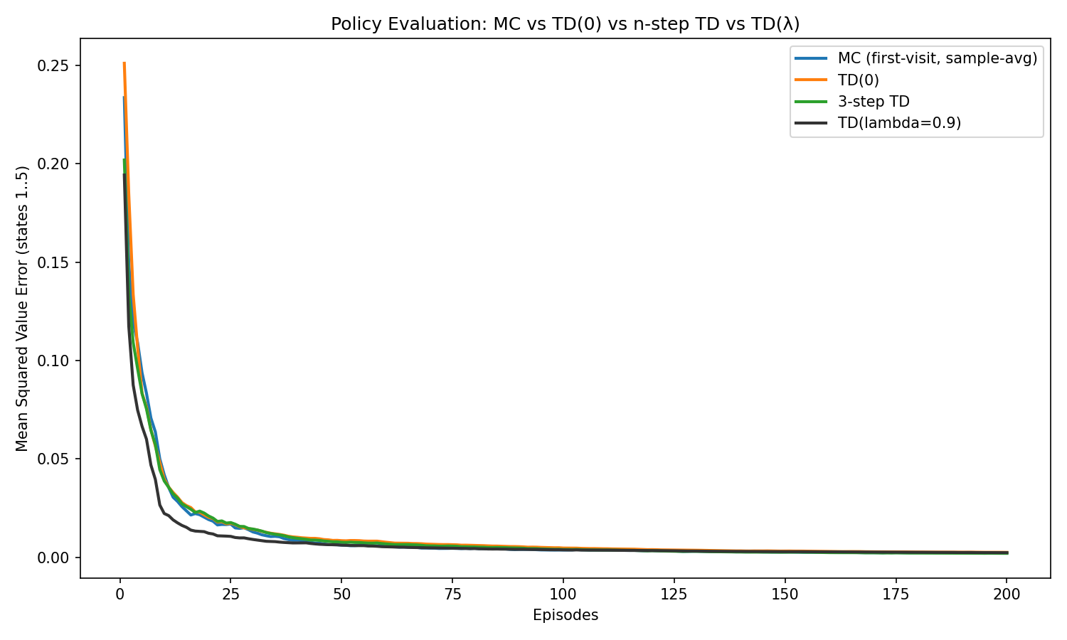
Figure 2.2: Policy Evaluation, MC versus TD Family, Diminishing Step Size

You are encouraged to play with the parameters of these algorithms in the code here.

2.1.2 Convergence Proof of TD Learning

Setup. Consider a tabular MDP with finite state space \(\mathcal{S}\) and action space \(\mathcal{A}\), and a discount factor \(\gamma \in [0,1)\). Assume the reward function is bounded, for example, \(R(s,a) \in [0,1]\) for any \((s,a) \in \mathcal{S} \times \mathcal{A}\). Let \(\pi\) be a stochastic policy and \(V^\pi\) be the true value function associated with \(\pi\), the target we wish to estimate from interaction data. Denote \[ \mathcal{F}_t = \sigma(s_0,a_0,r_0,\dots,s_{t-1},a_{t-1},r_{t-1}), \] as the \(\sigma\) algebra of all state-action-reward information up to time \(t-1\).

TD(0) Update. We maintain a tabular estimate \(V_t\) of the true value \(V^\pi\). On visiting \(s_t\) and observing \((s_t, a_t, r_t, s_{t+1})\), the TD(0) algorithm performs \[\begin{equation} V_{t+1}(s_t) = V_t(s_t) + \alpha_t(s_t) \delta_t, \tag{2.17} \end{equation}\] where \(\delta_t\) is the TD error \[ \delta_t = r_t + \gamma V_{t}(s_{t+1}) - V_t(s_t). \] The update (2.17) only changes the value at \(s_t\), leaving the value at other states unchanged.

Robbins–Monro Step Size. We assume the step size \(\alpha\) satisfy the Robbins–Monro condition. That is, for any \(s \in \mathcal{S}\): \[ \alpha_t(s) >0, \quad \sum_{t: s_t = s} \alpha_t(s) = \infty, \quad \sum_{t: s_t = s} \alpha^2_t(s) < \infty. \]

Stationary Distribution. Assume the Markov chain over \(\mathcal{S}\) induced by \(\pi\) is ergodic, then a unique stationary state distribution \(\mu^\pi\) exists and satisfy: \[\begin{equation} \mu^\pi(s') = \sum_{s \in \mathcal{S}} \mu^\pi(s) \left( \sum_{a \in \mathcal{A}} \pi(a \mid s) P(s' \mid s, a) \right), \quad \forall s' \in \mathcal{S}. \tag{2.18} \end{equation}\] If we denote \[\begin{equation} P^\pi(s' \mid s) = \sum_{a \in \mathcal{A}} \pi(a \mid s) P(s' \mid s,a), \tag{2.19} \end{equation}\] as the \(\pi\)-induced state-only transition dynamics, then condition (2.18) is equivalent to \[\begin{equation} \mu^\pi(s') = \sum_{s \in \mathcal{S}} \mu^\pi(s) P^\pi (s' \mid s), \quad \forall s' \in \mathcal{S}. \tag{2.20} \end{equation}\]

See (2.42) for a generalization to continuous MDP.

Bellman Operator. For any \(V:\mathcal S\to\mathbb R\), define the Bellman operator associated with \(\pi\) as \(T^\pi V:\mathcal S\to\mathbb R\) by \[\begin{equation} (T^\pi V)(s)\;=\;\sum_{a\in\mathcal A}\pi(a\mid s)\sum_{s'\in\mathcal S} P(s'\mid s,a)\,\Big( R(s,a)+\gamma\,V(s')\Big). \tag{2.21} \end{equation}\] We know that the operator \(T^\pi\) is a \(\gamma\)-contraction in \(\|\cdot\|_\infty\). Hence it has a unique fixed point \(V^\pi\) satisfying \(V^\pi=T^\pi V^\pi\).

The following theorem states the almost sure convergence of TD learning iterates to the true value function.

Theorem 2.1 (TD(0) Convergence (Tabular)) Under the tabular MDP setup and assumptions above, the TD(0) iterates \(V_t\) generated by (2.17) converge almost surely to \(V^\pi\).

To prove this theorem, we need the following two lemmas.

Lemma 2.1 (Robbins-Siegmund Lemma) Let \((X_t)_{t\ge 0}\) be nonnegative and adapted to \((\mathcal F_t)\). Suppose there exist nonnegative \((\beta_t),(\gamma_t),(\xi_t)\) with \(\sum_t \gamma_t<\infty\) and \(\sum_t \xi_t<\infty\) such that \[ \mathbb E[X_{t+1}\mid \mathcal F_t]\;\le\;(1+\gamma_t)X_t\;-\;\beta_t\;+\;\xi_t\qquad\text{almost surely} \] Then \(X_t\) converges almost surely to a finite random variable and \(\sum_t \beta_t<\infty\) almost surely.

This lemma is from (Robbins and Siegmund 1971).

Lemma 2.2 Let \(\mu^\pi\) be the stationary distribution in (2.20), \(D=\mathrm{diag}(\mu^\pi)\), and \(w:=V-V^\pi\). Then \[ \langle w,\,D\,(T^\pi V - V)\rangle\;\le\;-(1-\gamma)\,\|w\|_D^2, \] where \(\langle x,y\rangle=x^\top y\) and \(\|w\|_D^2=\sum_s \mu^\pi(s)\,w(s)^2\).

Proof. First, for any two value functions \(V, U \in \mathbb{R}^{|\mathcal{S}|}\), we have \[ (T^\pi V)(s) - (T^\pi U)(s) = \gamma \sum_{a} \pi(a \mid s) \sum_{s'} P(s' \mid s,a) (V(s') - U(s)'). \] Therefore, \[ T^\pi V - T^\pi U = \gamma \widetilde P (V - U), \] with \[\begin{equation} (\widetilde P u)(s):=\sum_a\pi(a\mid s)\sum_{s'}P(s'\mid s,a)\,u(s'). \tag{2.22} \end{equation}\] With this, we can write \[\begin{equation} \begin{split} T^\pi V - V & = T^\pi V - V^\pi + V^\pi - V \\ & = T^\pi V - T^\pi V^\pi - ( V - V^\pi ) \\ & = \gamma \widetilde P (V - V^\pi) - ( V - V^\pi ) \\ & = (\gamma \widetilde P - I) ( V - V^\pi ) \\ & = (\gamma \widetilde P - I) w. \end{split} \end{equation}\] Thus, \[\begin{equation} \langle w, D(T^\pi V - V)\rangle = -\,w^\top D\,(I-\gamma \widetilde P)\,w = -\|w\|_D^2 + \gamma\,\langle w, D\,\widetilde P w\rangle. \tag{2.23} \end{equation}\]

Next, we prove \(\langle w, D\widetilde P w\rangle\le \|w\|_D^2\).

• First, we show \(\|\widetilde P w\|_D\le \|w\|_D\). For any state \(s \in \mathcal{S}\), from (2.22), we have \[ (\widetilde P w)(s) = \sum_{s'} P^\pi (s' \mid s) w(s'), \] where \(P^\pi(s' \mid s)\) is the \(\pi\)-induced state-only transition in (2.19). Since \(P^\pi(\cdot \mid s)\) is a probability distribution, and \(x \mapsto x^2\) is convex, we have \[ ((\widetilde P w)(s))^2 = \left( \sum_{s'} P^\pi (s' \mid s) w(s') \right)^2 \leq \sum_{s'} P^\pi (s' \mid s) w^2(s'). \] Therefore, we have \[\begin{equation} \begin{split} \Vert \widetilde P w \Vert_D^2 & = \sum_s \mu^{\pi}(s) ((\widetilde P w)(s))^2 \\ & \leq \sum_s \mu^{\pi}(s) \left( \sum_{s'} P^\pi (s' \mid s) w^2(s') \right) \\ & = \sum_{s'} \left( \sum_{s} \mu^\pi(s) P^\pi(s' \mid s) \right) w^2(s') \\ & = \sum_{s'} \mu^\pi (s') w^2 (s') = \Vert w \Vert_D^2. \end{split} \end{equation}\] where the second-from-last equality holds because \(\mu^\pi\) is the stationary distribution and satisfies (2.20).

• Second, we write \[ \langle w, D\widetilde P w\rangle = \langle D^{0.5} w, D^{0.5} \widetilde P w \rangle \leq \Vert D^{0.5} w \Vert \cdot \Vert D^{0.5} \widetilde P w \Vert = \Vert w \Vert_D \cdot \Vert \widetilde P w \Vert_D \leq \Vert w \Vert_D^2. \]

Plugging this back to (2.23), we obtain \[ \langle w, D(T^\pi V - V) \rangle \leq - \Vert w \Vert_D^2 + \gamma \Vert w \Vert_D^2, \] proving the desired result in the lemma.

We are now ready to prove Theorem 2.1.

Proof. Step 1 (TD as stochastic approximation). For the TD error \[ \delta_t=r_{t}+\gamma V_t(s_{t+1})-V_t(s_t), \] we have the conditional expectation \[ \mathbb E[\delta_t\mid \mathcal F_t, s_t] =\sum_{a}\pi(a\mid s_t)\sum_{s'}P(s'\mid s_t,a)\Big(R(s_t,a)+\gamma V_t(s')\Big)-V_t(s_t) =\big(T^\pi V_t - V_t\big)(s_t). \] Define the “noise”: \[ \eta_{t+1}:=\delta_t-\mathbb E[\delta_t\mid \mathcal F_t,s_t]. \] Then \(\mathbb E[\eta_{t+1}\mid \mathcal F_t,s_t]=0\) and the TD update is equivalent to \[\begin{equation} V_{t+1}(s_t)=V_t(s_t)+\alpha_t(s_t)\Big( \big(T^\pi V_t - V_t\big)(s_t) + \eta_{t+1}\Big), \tag{2.24} \end{equation}\] while learving all other coordinates unchanged. Because rewards are uniformly bounded, we know that \(V_t\) remains bounded. Hence, \(\mathbb E[\eta_{t+1}^2\mid \mathcal F_t, s_t]\) is uniformly bounded. Equation (2.24) shows that the TD update can be seen as a stochastic approximation to the Bellman operator (2.21).

Step 2 (Lyapunov drift). Let \(D=\mathrm{diag}(\mu^\pi)\), a diagonal matrix whose diagonal entries are the probabilities in \(\mu^\pi\). Define the Lyapunov function \[ \mathcal L(V)=\frac{1}{2} \|V-V^\pi\|_D^2=\frac{1}{2} \sum_s \mu^\pi(s)\,\big(V(s)-V^\pi(s)\big)^2. \] Let \(w_t:=V_t - V^\pi\). Since only the \(s_t\)-coordinate changes at time \(t\), we have \[\begin{equation} \begin{split} \mathcal L(V_{t+1})-\mathcal L(V_t) &=\frac{1}{2} \mu^\pi(s_t)\Big(( \underbrace{V_t(s_t)+\alpha_t\delta_t}_{V_{t+1}(s_t)} - V^\pi(s_t) )^2 -(V_t(s_t)-V^\pi(s_t))^2\Big)\\ &= \mu^\pi(s_t)\,\alpha_t\,\delta_t\,w_t(s_t)\;+\;\frac{1}{2} \mu^\pi(s_t)\,\alpha_t^2\,\delta_t^{\,2}. \end{split} \tag{2.25} \end{equation}\] Define \(g_t := T^\pi V_t - V_t\). Taking conditional expectation given \(\mathcal F_t\) and i.i.d. \(s_t\sim \mu^\pi\), \[\begin{equation} \begin{split} \mathbb E\!\left[\mathcal L(V_{t+1})-\mathcal L(V_t)\mid \mathcal F_t\right] &= \alpha_t\,\mathbb E\!\left[\mu^\pi(s_t)\,w_t(s_t)\,g_t(s_t)\mid \mathcal F_t\right] + \frac{1}{2} \alpha_t^2\,\mathbb E\!\left[\mu^\pi(s_t)\,\delta_t^{\,2}\mid \mathcal F_t\right]\\ &= \alpha_t\,\sum_s \mu^\pi(s)\,w_t(s)\,g_t(s) \;+\; \frac{1}{2} \alpha_t^2\,C_t, \end{split} \tag{2.26} \end{equation}\] where \(C_t:=\mathbb E\!\left[\mu^\pi(s_t)\,\delta_t^{\,2}\mid \mathcal F_t\right]\) is finite because rewards are bounded and \(V_t\) stays bounded. Assume \(C_t \leq C\).

At the same time, by Lemma 2.2 \[ \sum_s \mu^\pi(s)\,w_t(s)\,g_t(s) =\langle w_t, D g_t\rangle \le -(1-\gamma)\,\|w_t\|_D^2. \] Plugging into (2.26) yields \[\begin{equation} \mathbb E\!\left[\mathcal L(V_{t+1})\mid \mathcal F_t\right] \;\le\; \mathcal L(V_t)\;-\;\alpha_t\,(1-\gamma)\,\|w_t\|_D^2\;+\;\frac{1}{2} \alpha_t^2\,C. \tag{2.27} \end{equation}\] This is in Robbins–Siegmund form with \[ X_t:=\mathcal L(V_t),\qquad \beta_t:=(1-\gamma)\,\alpha_t\,\|w_t\|_D^2,\qquad \gamma_t:=0,\qquad \xi_t:=\frac{1}{2} C\,\alpha_t^2. \] We have \(\sum_t \xi_t<\infty\) by \(\sum_t \alpha_t^2<\infty\). Therefore \(X_t\) converges a.s. and \(\sum_t \beta_t<\infty\) a.s., which implies \(\sum_t \alpha_t \|w_t\|_D^2<\infty\). Since \(\sum_t \alpha_t=\infty\), it must be that \(\liminf_t \|w_t\|_D=0\).
Finally, using (2.27) again and the continuity of the drift, one shows that any subsequential limit of \(V_t\) must satisfy \(T^\pi V - V=0\); by uniqueness of the fixed point, the only possible limit is \(V^\pi\). Hence \(V_t\to V^\pi\) almost surely.

2.1.3 On-Policy Control

Monte Carlo (MC) estimation and the TD family evaluate policies directly from interaction—no model required. We now turn evaluation into control via generalized policy iteration (GPI): repeatedly (i) evaluate the current policy from data and (ii) improve it by acting greedily with respect to the new estimates. We first cover on-policy control methods, which estimate and improve the same (typically \(\varepsilon\)-greedy) policy, and then off-policy methods, which learn about a target policy while behaving with a different one.

2.1.3.1 Monte Carlo Control

High-level Intuition.

• Goal. Learn an (approximately) optimal policy by alternating policy evaluation and policy improvement using only sampled episodes.

• Why action-values? Estimating \(Q^\pi(s,a)\) lets us improve the policy without a model by choosing “\(\arg\max_a Q(s,a)\)”.

• Exploration. Pure greedy improvement can get stuck. MC control keeps the policy \(\varepsilon\)-soft (e.g., \(\varepsilon\)-greedy) so that every action has nonzero probability and all state-action pairs continue to be sampled. An \(\varepsilon\)-soft policy is one that never rules out any action: in every state \(s\), each action \(a\) gets at least a small fraction of probability. Formally, in the tabular setup, we have that a policy \(\pi\) is \(\varepsilon\)-soft if and only if \[\begin{equation} \forall s, \forall a: \quad \pi(a \mid s) \geq \frac{\varepsilon}{|\mathcal{A}(s)|}, \quad \varepsilon \in (0,1], \tag{2.28} \end{equation}\] where \(\mathcal{A}(s)\) denotes the set of actions the agent can select at state \(s\).

• Coverage mechanisms. Classic guarantees use either:

  1. Exploring starts (ES): start each episode from a randomly chosen \((s,a)\) with nonzero probability; or
     
  2. \(\varepsilon\)-soft / GLIE (Greedy in the Limit with Infinite Exploration): use \(\varepsilon\)-greedy behavior with \(\varepsilon_t \downarrow 0\) so every \((s,a)\) is visited infinitely often while the policy becomes greedy in the limit.

Algorithmic Form. We maintain tabular action-value estimates \(Q(s,a)\) and an \(\varepsilon\)-soft policy \(\pi\) (\(\varepsilon\)-greedy w.r.t. \(Q\)). After each episode we update \(Q\) from empirical returns and then improve \(\pi\).

Return from time \(t\): \[ g_t = r_t + \gamma r_{t+1} + \dots + \gamma^{T-t} r_T = \sum_{k=0}^{T-t} \gamma^{k} r_{t+k}. \]

First-visit MC update (common choice): \[\begin{equation} Q(s_t,a_t) \;\leftarrow\; Q(s_t,a_t) + \alpha_{N(s_t,a_t)}\!\left(g_t - Q(s_t,a_t)\right), \tag{2.29} \end{equation}\] applied only on the first occurrence of \((s_t,a_t)\) in the episode. Sample-average learning uses \(\alpha_n = 1/n\) per pair; more generally, use diminishing stepsizes.

Policy improvement (\(\varepsilon\)-greedy): \[\begin{equation} \pi(a|s) \;=\; \begin{cases} 1-\varepsilon + \dfrac{\varepsilon}{|\mathcal{A}(s)|}, & a \in \arg\max_{a'} Q(s,a'), \\ \dfrac{\varepsilon}{|\mathcal{A}(s)|}, & \text{otherwise}. \end{cases} \tag{2.30} \end{equation}\]

Theoretical Guarantees.

Assume a tabular episodic MDP and \(\gamma \in [0,1)\).

• Convergence with Exploring Starts. If every state–action pair has nonzero probability of being the first pair of an episode (using ES), and each \(Q(s,a)\) is updated toward the true mean return from \((s,a)\) (e.g., via sample averages), then repeated policy evaluation and greedy improvement converge with probability 1 to an optimal deterministic policy. (If one uses an \(\varepsilon\)-greedy improvement, then it converges to an optimal \(\varepsilon\)-soft policy.)

• Convergence with \(\varepsilon\)-soft GLIE behavior. If the behavior policy is GLIE—every \((s,a)\) is visited infinitely often and \(\epsilon_t \to 0\)—and the stepsizes for each \((s,a)\) satisfy the Robbins–Monro conditions \(\sum_{t} \alpha_t(s,a) = \infty,\sum_{t} \alpha_t(s,a)^2 < \infty\), then \(Q(s,a)\) converges to \(Q^\star(s,a)\) for all pairs visited infinitely often, and the \(\varepsilon\)-greedy policy converges almost surely to an optimal policy.

Remark. Unbiased but high-variance. MC targets \(g_t\) are unbiased estimates of action values under the current policy, but can have high variance—especially for long horizons—so convergence can be slower than TD methods. Keeping \(\varepsilon>0\) ensures exploration but limits asymptotic optimality to the best \(\varepsilon\)-soft policy; hence \(\varepsilon_t \downarrow 0\) (GLIE) is recommended for optimality.

2.1.3.2 SARSA (On-Policy TD Control)

High-level Intuition.

• Goal. Turn evaluation into control by updating action values online and improving the same policy that generates data.
• Key idea. Replace Monte Carlo returns with a bootstrapped target. After taking action \(a_t\) in state \(s_t\) and observing \(r_{t}, s_{t+1}\), sample the next action \(a_{t+1}\) from the current policy and update toward \(r_{t} + \gamma Q(s_{t+1}, a_{t+1})\).
• On-policy nature. SARSA evaluates the behavior policy itself, typically an \(\varepsilon\)-greedy policy w.r.t. \(Q\).
• Exploration. Use \(\varepsilon\)-soft behavior so every action keeps nonzero probability. For optimality, let \(\varepsilon_t \downarrow 0\) to obtain GLIE (Greedy in the Limit with Infinite Exploration).

Algorithmic Form.

Let \(Q\) be a tabular action-value function and \(\pi_t\) be \(\varepsilon_t\)-greedy w.r.t. \(Q_t\).

TD target and error: \[\begin{equation} y_t = r_{t} + \gamma Q(s_{t+1}, a_{t+1}), \qquad \delta_t = y_t - Q(s_t, a_t). \tag{2.31} \end{equation}\]

SARSA update (one-step): \[\begin{equation} Q(s_t, a_t) \leftarrow Q(s_t, a_t) + \alpha_t(s_t,a_t)\, \delta_t. \tag{2.32} \end{equation}\]

\(\varepsilon\)-greedy policy improvement: \[\begin{equation} \pi_{t+1}(a\mid s) = \begin{cases} 1-\varepsilon_{t+1} + \dfrac{\varepsilon_{t+1}}{|\mathcal A(s)|}, & a \in \arg\max_{a'} Q_{t+1}(s,a'),\\ \dfrac{\varepsilon_{t+1}}{|\mathcal A(s)|}, & \text{otherwise.} \end{cases} \tag{2.33} \end{equation}\]

Variants.

• Expected SARSA replaces the sampled \(a_{t+1}\) by its expectation under \(\pi_t\) for lower variance: \[\begin{equation} y_t = r_{t} + \gamma \sum_a \pi_t(a\mid s_{t+1}) Q(s_{t+1}, a). \tag{2.34} \end{equation}\]

• \(n\)-step SARSA and SARSA(\(\lambda\)) blend multi-step targets; these trade bias and variance similarly to MC vs TD.

Convergence Guarantees.

Assume a finite MDP, \(\gamma \in [0,1)\), asynchronous updates, and that each state–action pair is visited infinitely often.

• GLIE convergence to optimal policy. If the behavior is GLIE, i.e., \(\varepsilon_t \downarrow 0\) while ensuring infinite exploration, and stepsizes satisfy the Robbins–Monro conditions, then \(Q_t \to Q^\star\) almost surely and the \(\varepsilon_t\)-greedy behavior becomes greedy in the limit, yielding an optimal policy almost surely.

2.1.4 Off-Policy Control

Off-policy methods learn about a target policy \(\pi\) while following a (potentially different) behavior policy \(b\) to gather data. This decoupling is useful when:

• you want to reuse logged data collected by some \(b\) (e.g., a rule-based controller or a past system),

• you need safer exploration by restricting behavior \(b\) while aiming to evaluate or improve a different \(\pi\),

• you want to learn about the greedy policy without executing it, which motivates algorithms like Q-learning.

In this section we first cover off-policy policy evaluation with importance sampling, then show how it can be used to construct an off-policy Monte Carlo control scheme in the tabular case. Finally, we present Q-learning.

2.1.4.1 Importance Sampling for Policy Evaluation

Motivation. Suppose we have episodes generated by a behavior policy \(b\), but we want the value of a different target policy \(\pi\). For a state value this is \(V^\pi(s) = \mathbb{E}_\pi[g_t \mid s_t=s]\), and for action values \(Q^\pi(s,a) = \mathbb{E}_\pi[g_t \mid s_t=s, a_t=a]\), where \[ g_t = \sum_{k=0}^{T-t} \gamma^{k} r_{t+k}. \] Because the data come from \(b\), the naive sample average is biased. Importance sampling (IS) reweights returns so that expectations under \(b\) equal those under \(\pi\).

A basic support condition is required: \[\begin{equation} \text{If } \pi(a\mid s) > 0 \text{ then } b(a\mid s) > 0 \quad \text{for all visited } (s,a). \tag{2.35} \end{equation}\] This ensures that \(\pi\) is absolutely continuous with respect to \(b\) on the experienced trajectories.

Importance Sampling (episode-wise). Consider a trajectory starting at time \(t\): \[ \tau_t = (s_t, a_t, r_t, s_{t+1}, a_{t+1}, \dots, s_{T-1}, a_{T-1}, r_{T-1}, s_T). \] The probability of observing this trajectory conditioned on \(s_t = s\), under policy \(\pi\), is \[ \mathbb{P}_{\pi}[\tau_t \mid s_t = s] = \pi(a_t \mid s_t) P(s_{t+1} \mid s_t, a_t) \pi(a_{t+1} \mid s_{t+1}) \cdots \pi(a_{T-1} \mid s_{T-1}) P(s_T \mid s_{T-1}, a_{T-1}). \] The probability of observing the same trajectory conditioned on \(s_t = s\), under policy \(b\), is \[ \mathbb{P}_{b}[\tau_t \mid s_t = s] = b(a_t \mid s_t) P(s_{t+1} \mid s_t, a_t) b(a_{t+1} \mid s_{t+1}) \cdots b(a_{T-1} \mid s_{T-1}) P(s_T \mid s_{T-1}, a_{T-1}). \] Since the return \(g_t\) is a deterministic function of \(\tau_t\), i.e., applying the reward function \(R\) to state-action pairs, we have that \[\begin{equation} \begin{split} V^\pi (s) & = \mathbb{E}_{\pi}[g_t \mid s_t = s] = \sum_{\tau_t} g_t \mathbb{P}_\pi [\tau_t \mid s_t = s] \\ & = \sum_{\tau_t} g_t \mathbb{P}_b[\tau_t \mid s_t = s] \left(\frac{\mathbb{P}_\pi [\tau_t \mid s_t = s]}{\mathbb{P}_b[\tau_t \mid s_t = s]} \right) \\ & = \sum_{\tau_t} \left( \frac{\pi(a_t \mid s_t) \pi(a_{t+1} \mid s_{t+1}) \cdots \pi(a_{T-1} \mid s_{T-1}) }{b(a_t \mid s_t) b(a_{t+1} \mid s_{t+1}) \cdots b(a_{T-1} \mid s_{T-1})} \right) g_t \mathbb{P}_b [\tau_t \mid s_t = s] \end{split} \tag{2.36} \end{equation}\] Therefore, define the likelihood ratio \[\begin{equation} \rho_{t:T-1} = \prod_{k=t}^{T-1} \frac{\pi(a_k \mid s_k)}{b(a_k \mid s_k)}, \tag{2.37} \end{equation}\] we have \[\begin{equation} V^\pi(s) = \mathbb{E}_b\left[\rho_{t:T-1} g_t \mid s_t=s\right]. \tag{2.38} \end{equation}\] Similarly, we have \[\begin{equation} Q^\pi(s,a) = \mathbb{E}_b\!\left[\rho_{t:T-1} g_t \mid s_t=s, a_t=a\right]. \tag{2.39} \end{equation}\] Given \(n\) episodes, the ordinary IS estimator for \(Q^\pi\) at the first visit of \((s,a)\) is \[ \hat Q_n^{\text{IS}}(s,a) = \frac{1}{N_n(s,a)} \sum_{i=1}^n \mathbf{1}\{(s,a)\text{ visited}\}\, \rho_{t_i:T_i-1}^{(i)}\, g_{t_i}^{(i)}, \] where \(N_n(s,a)\) counts the number of first visits of \((s,a)\). In words, to estimate the \(Q\) value of the target policy \(\pi\) using trajectories of the behavior policy \(b\), we need to reweight the return \(g_t\) by the likelihood ratio \(\rho_{t:T-1}\). Note that the likelihood ratio does not require knowledge about the transition dynamics.

Algorithmic Form: Off-policy Monte Carlo Policy Evaluation.

Input: behavior \(b\), target \(\pi\), episodes from \(b\)
For each episode \((s_0,a_0,r_0,s_1,\dots,s_{T-1},a_{T-1},r_{T-1},s_T)\):

1. For \(t=T-1,\dots,0\) compute episode-wise likelihood ratio \(\rho_{t:T-1}\) and return \(g_t\),

2. For first visits of \((s_t,a_t)\), update \[ Q(s_t,a_t) \leftarrow Q(s_t,a_t) + \alpha_{N(s_t,a_t)}\big(\rho_{t:T-1} g_t - Q(s_t,a_t)\big). \] Use sample averages \(\alpha_n=1/n\) or Robbins-Monro stepsizes.

Guarantees. Under the support condition and finite variance assumptions, ordinary IS is unbiased and converges almost surely to \(Q^\pi\).

2.1.4.2 Off-Policy Monte Carlo Control

High-level Intuition. We wish to improve a target policy \(\pi\) toward optimality while behaving with a different exploratory policy \(b\). We evaluate \(Q^\pi\) off-policy using IS on data from \(b\), then set \(\pi\) greedy with respect to the updated \(Q\). Keep \(b\) sufficiently exploratory (for coverage), for example \(\varepsilon\)-greedy with a fixed \(\varepsilon>0\) or a GLIE schedule.

Algorithmic Form.

1. Initialize \(Q(s,a)\) arbitrarily. Set target \(\pi\) to be greedy w.r.t. \(Q\). Choose an exploratory behavior \(b\) that ensures coverage, e.g., \(\varepsilon\)-greedy w.r.t. \(Q\) with \(\varepsilon>0\).

2. Loop over iterations \(i=0,1,2,\dots\):

   1. Data collection under \(b\): generate a batch of episodes using \(b\).
   2. Off-policy evaluation of \(\pi\): for each episode, compute IS targets for first visits of \((s_t,a_t)\) and update \(Q\) using either ordinary IS
   3. Policy improvement: set for all states \[ \pi_{i+1}(s) \in \arg\max_{a} Q(s,a). \]
   4. Optionally update \(b\) to remain exploratory, for example \(b\) \(\leftarrow\) \(\varepsilon\)-greedy w.r.t. \(Q\) with a chosen \(\varepsilon\) or a GLIE decay.

Convergence Guarantees.

• Evaluation step: With the support condition and appropriate stepsizes, off-policy MC prediction converges almost surely to \(Q^\pi\) when using ordinary IS.

• Control in the batch GPI limit: If each evaluation step produces estimates that converge to the exact \(Q^{\pi_i}\) before improvement, then by the policy improvement theorem the sequence of greedy target policies \(\pi_i\) converges to an optimal policy in finite MDPs.

Remark. Choice of \(b\). A common and simple choice is an \(\varepsilon\)-greedy behavior \(b\) w.r.t. current \(Q\) that maintains \(\varepsilon>0\) for coverage or uses GLIE so that \(\varepsilon_t \downarrow 0\) while all pairs are still visited infinitely often.

2.1.4.3 Q-Learning

High-Level Intuition.

• What it learns. Q-Learning seeks the fixed point of the Bellman optimality operator \[ (\mathcal T^\star Q)(s,a) = \mathbb E\big[ r_{t} + \gamma \max_{a'} Q(s_{t+1}, a') \mid s_t=s, a_t=a \big], \] whose unique fixed point is \(Q^\star\). Because \(\mathcal T^\star\) is a \(\gamma\)-contraction in \(\|\cdot\|_\infty\), repeatedly applying it converges to \(Q^\star\) in the tabular case.

• Why off-policy. We can behave with any sufficiently exploratory policy \(b\) (e.g., \(\varepsilon\)-greedy w.r.t. current \(Q\)) but learn from the greedy target \(\max_{a'} Q(s',a')\). No importance sampling is needed.

Algorithmic Form. Let \(Q\) be a tabular action-value function. At each step observe a transition \((s_t, a_t, r_{t}, s_{t+1})\) generated by a behavior policy \(b_t\) (typically \(\varepsilon_t\)-greedy w.r.t. \(Q_t\)).

• Target and TD error \[ y_t = r_{t} + \gamma \max_{a'} Q(s_{t+1}, a'), \qquad \delta_t = y_t - Q(s_t, a_t). \]

• Update \[ Q(s_t, a_t) \leftarrow Q(s_t, a_t) + \alpha_t(s_t,a_t)\, \delta_t. \]

• Behavior (exploration) Use \(\varepsilon_t\)-greedy with \(\varepsilon_t\) decaying (GLIE) or any scheme that ensures each \((s,a)\) is updated infinitely often.

Convergence. In a finite MDP with \(\gamma \in [0,1)\), if each \((s,a)\) is updated infinitely often (sufficient exploration) and stepsizes satisfy Robbins-Monro conditions, then Q-Learning converges to \(Q^\star\) with probability 1.

2.1.4.4 Double Q-Learning

Motivation. Max operators tend to be optimistically biased when action values are noisy. Consider an example where in state \(s\) one can take two actions \(1\) and \(2\). The estimated Q function \(\hat{Q}(s, \cdot)\) has two values \(+1\) and \(-1\) with equal probability. In this case we have \(Q(s,1) = Q(s,2) = \mathbb{E}[\hat{Q}(s,\cdot)] = 0\). Therefore, \(\max Q(s,a) = 0\). However, the noisy estimated \(\hat{Q}(s,\cdot)\) has four outcomes with equal probabilities: \[ (+1,-1), (+1,+1), (-1, +1), (-1,-1). \] Therefore, we have \[ \mathbb{E}[\max_a \hat{Q}(s,a)] = \frac{1}{4} (1 + 1 + 1 -1) = 1/2 > \max_a Q(s,a), \] which overestimates the max \(Q\) value. In general, we have \[ \mathbb{E}[\max_a \hat{Q}(s,a)] \geq \max_a \mathbb{E} [\hat{Q}(s,a)] = \max_a Q(s,a), \] where the estimates \(\hat{Q}\) are noisy (try to prove this on your own). In Q-Learning the target \[ y_t = r_{t} + \gamma \max_{a'} Q(s_{t+1}, a') \] can therefore overestimate action values and slow learning or push policies toward risky actions.

Double Q-Learning reduces this bias by decoupling selection from evaluation: maintain two independent estimators \(Q^A\) and \(Q^B\). Use one to select the greedy action and the other to evaluate it, and alternate which table you update. This weakens the statistical coupling that creates overestimation.

Algorithmic Form. Keep two tables \(Q^A, Q^B\). Use an \(\varepsilon\)-greedy behavior policy with respect to a combined estimate, e.g., \(Q^{\text{avg}}= \tfrac12(Q^A+Q^B)\) or \(Q^A+Q^B\).

At each step observe \((s_t, a_t, r_{t}, s_{t+1})\). With probability \(1/2\) update \(Q^A\), else update \(Q^B\).

• Update \(Q^A\): \[ a^\star = \arg\max_{a'} Q^A(s_{t+1}, a'),\qquad y_t = r_{t} + \gamma\, Q^B(s_{t+1}, a^\star), \] \[ Q^A(s_t, a_t) \leftarrow Q^A(s_t, a_t) + \alpha_t(s_t,a_t)\big[y_t - Q^A(s_t, a_t)\big]. \]

• Update \(Q^B\): \[ a^\star = \arg\max_{a'} Q^B(s_{t+1}, a'),\qquad y_t = r_{t} + \gamma\, Q^A(s_{t+1}, a^\star), \] \[ Q^B(s_t, a_t) \leftarrow Q^B(s_t, a_t) + \alpha_t(s_t,a_t)\big[y_t - Q^B(s_t, a_t)\big]. \]

• Behavior policy (\(\varepsilon\)-greedy): choose \(a_t \sim \varepsilon\)-greedy with respect to \(Q^{\text{avg}}(s_t,\cdot)\). A GLIE schedule \(\varepsilon_t \downarrow 0\) is standard.

• Acting and planning: for greedy actions or plotting a single estimate, use \(Q^{\text{avg}} = \tfrac12(Q^A+Q^B)\).

Convergence.

• Tabular setting. In a finite MDP with \(\gamma \in [0,1)\), bounded rewards, sufficient exploration so that every \((s,a)\) is updated infinitely often, and Robbins–Monro stepsizes for each pair. Double Q-Learning converges with probability 1 to \(Q^\star\).

Example 2.2 (Value-based RL for Grid World) Consider the following \(5 \times 5\) grid with \((0,4)\) being the goal and the terminal state. At every state, the agent can take four actions: left, right, up, and down. There is a wall in the gray area shown in Fig. 2.3. Upon hitting the wall, the agent stays in the original cell. Every action incurs a reward of \(-1\). Once the agent arrives at the goal state, reward stays at 0.

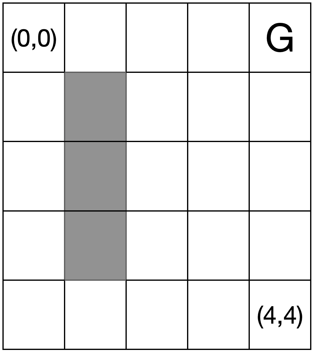
Figure 2.3: Grid World

We run Generalized Policy Iteration (GPI) with Monte Carlo (on-policy), SARSA, Expected SARSA, Q-Learning, and Double Q-Learning on this problem with diminishing learning rates.

Fig. 2.4 plots the error between the estimated Q values (of different algorithms) and the ground-truth optimal Q value (obtained from value iteration with known transition dynamics). Except Monte Carlo control which converges slowly, the other methods converge fast.

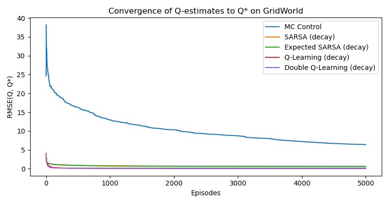
Figure 2.4: Convergence of Estimated Q Values.

From the final estimated Q value, we can extract a greedy policy, visualized below.

You can play with the code here.

MC Control:
 > > > > G
^ # ^ ^ ^
v # ^ ^ ^
v # > ^ ^
> > > > ^
SARSA:
 > > > > G
^ # > > ^
^ # ^ ^ ^
^ # ^ ^ ^
> > ^ ^ ^
Expected SARSA:
 > > > > G
^ # > > ^
^ # ^ ^ ^
^ # > > ^
> > ^ ^ ^
Q-Learning:
 > > > > G
^ # ^ ^ ^
^ # ^ ^ ^
^ # ^ ^ ^
> > ^ ^ ^
Double Q-Learning:
 > > > > G
^ # > ^ ^
^ # > ^ ^
^ # ^ ^ ^
> > > > ^

2.2 Function Approximation

Many reinforcement learning problems have continuous state spaces–think of mechanical systems like robot arms, legged locomotion, drones, and autonomous vehicles. In these domains the state \(s\) (e.g., joint angles/velocities, poses) lives in \(\mathbb{R}^n\), which makes a tabular representation of the value functions impossible. In this case, we must approximate values with parameterized functions.

2.2.1 Basics of Continuous MDP

In a continuous MDP, at least one of the state space or the action space is a continuous space. Suppose \(\mathcal{S} \subseteq \mathbb{R}^n\) and \(\mathcal{A} \subseteq \mathbb{R}^{m}\) are both continuous spaces.

The environment kernel \(P(\cdot \mid s, a)\) is a Markov kernel from \(\mathcal{S} \times \mathcal{A}\) to \(\mathcal{S}\): for each state-action pair \((s,a)\), \(P(\cdot \mid s,a)\) is a probability measure on \(\mathcal{S}\). For each Borel set \(B \subseteq \mathcal{S}\), the map \((s,a) \mapsto P(B \mid s, a)\) is measurable. For example, \(P(\mathcal{S} \mid s, a) = 1\) for any \((s,a)\).

The policy kernel \(\pi(\cdot \mid s)\) is a stochastic kernel from \(\mathcal{S}\) to \(\mathcal{A}\): for each \(s\), \(\pi(\cdot \mid s)\) is a probability measure on \(\mathcal{A}\).

Induced State-Transition Kernel. For notational convenience, given a policy and the environment kernel \(P\), we define a state-only Markov kernel \[\begin{equation} P^\pi(B \mid s) := \int_{\mathcal{A}} P(B \mid s, a) \pi(da \mid s), \quad B \subseteq \mathcal{S}. \tag{2.40} \end{equation}\] In words, \(P^\pi(B \mid s)\) measures the probability of landing at a set \(B\) starting from state \(s\), under all actions possible for the policy \(\pi\).

If densities exist, i.e., \(P(ds' \mid s, a) = p(s' \mid s, a) ds'\) and \(\pi(da \mid s) = \pi(a \mid s) da\), then, \[\begin{equation} p^\pi(s' \mid s) := \int_{\mathcal{A}} p(s' \mid s, a) \pi(a \mid s) da \quad\text{and}\quad P^{\pi}(d s' \mid s) = p^\pi(s' \mid s) ds'. \tag{2.41} \end{equation}\]

Stationary State Distribution. A probability measure \(\mu^\pi\) on \(\mathcal{S}\) is called stationary for the state-transition kernel \(P^\pi\) if and only if \[\begin{equation} \mu^{\pi}(B) = \int_{\mathcal{S}} P^\pi(B \mid s) \mu^{\pi}(ds), \quad \forall B \subseteq \mathcal{S}. \tag{2.42} \end{equation}\] If a density \(\mu^\pi(s)\) exists, then the above equation is the followng condition \[\begin{equation} \mu^{\pi}(s') = \int_{\mathcal{S}} p^\pi(s' \mid s) \mu^{\pi}(s) ds. \tag{2.43} \end{equation}\] In words, the state distribution \(\mu^\pi\) does not change under the state-transition kernel \(P^\pi\) (e.g., if a state \(A\) has probability \(0.1\) of being visited at time \(t\), the probability of visiting \(A\) in the next time step remains \(0.1\), under policy \(\pi\)). Under standard ergodicity assumptions, this stationary state distribution \(\mu^\pi\) exists and is unique (after sufficient steps, the initial state distribution does not matter and the state distribution follows \(\mu^\pi\)). Moreover, the empirical state distribution converge to \(\mu^\pi\).

2.2.2 Policy Evaluation

For simplicity, let us first relax the state space to be a continuous space \(\mathcal{S} \subseteq \mathbb{R}^n\). We assume the action space \(\mathcal{A}\) is still finite with \(|\mathcal{A}|\) elements. We first consider the problem of policy evaluation, i.e., estimate the value functions associated with a policy \(\pi\) from interaction data with the environment.

Bellman Consistency. Given a policy \(\pi: \mathcal{S} \mapsto \Delta(\mathcal{A})\), its associated state-value function \(V^\pi\) must satisfy the following Bellman Consistency equation \[\begin{equation} V^{\pi}(s) = \sum_{a \in \mathcal{A}} \pi(a \mid s) \left[ R(s, a) + \gamma \int_{\mathcal{S}} V(s') P(d s' \mid s, a) \right]. \tag{2.44} \end{equation}\] Notice that since \(\mathcal{S}\) is a continuous space, we need to replace “\(\sum_{s' \in \mathcal{S}}\)” with “\(\int_{\mathcal{S}}\)”. If \(P(d s' \mid s, a)\) has a density \(p(s' \mid s, a)\), the above Bellman consistency equation also reads \[\begin{equation} V^{\pi}(s) = \sum_{a \in \mathcal{A}} \pi(a \mid s) \left[ R(s, a) + \gamma \int_{\mathcal{S}} V(s') p(s' \mid s, a) ds' \right]. \tag{2.45} \end{equation}\]

Bellman Operator. Define the Bellman operator \(T^\pi\) acting on any bounded measurable function \(V:\mathcal{S}\to\mathbb{R}\) by \[\begin{equation} (T^\pi V)(s) = \sum_{a\in\mathcal{A}} \pi(a\mid s)\left[ R(s,a) + \gamma \int_{\mathcal{S}} V(s') P(ds'\mid s,a)\right]. \tag{2.46} \end{equation}\] Then \(V^\pi\) is the unique fixed point of \(T^\pi\), i.e., \(V^\pi = T^\pi V^\pi\). Moreover, when rewards are uniformly bounded and \(\gamma\in[0,1)\), \(T^\pi\) is a \(\gamma\)-contraction under the sup-norm and is monotone.

Approximate Value Function. In large/continuous state spaces we restrict attention to a parametric family \({V(\cdot;\theta): \theta\in\mathbb{R}^d}\) and learn \(\theta\) from data. We use \(\nabla_\theta V(s;\theta) \in \mathbb{R}^d\) to denote the gradient of \(V\) with respect to \(\theta\) at state \(s\).

A special and very important case is linear function approximation \[\begin{equation} V(s;\theta) = \theta^\top \phi(s), \tag{2.47} \end{equation}\] where \(\phi(s) = [\phi_1(s),\ldots,\phi_d(s)]^\top\) are fixed basis functions (e.g., neural network last-layer features). When \(V(s;\theta) = \theta^{\top} \phi(s)\), we have \[ \nabla_\theta V(s;\theta) = \phi(s). \] When we restrict the value function to a function class (e.g., linear features or a neural network), it is generally not guaranteed that the unique fixed point of the Bellman operator (2.46), namely \(V^\pi\), belongs to that class. This misspecification (or realizability gap) means we typically cannot recover \(V^\pi\) exactly; instead, we seek its best approximation according to a chosen criterion.

2.2.2.1 Monte Carlo Estimation

Given an episode \((s_t,a_t,r_t,\dots,s_T)\) collected by policy \(\pi\), its discounted return \[ g_t = r_t + \gamma r_{t+1} + \gamma^2 r_{t+2} + \dots + \gamma^{T-t} r_T \] is an unbiased estimate of the value at \(s_t\), i.e., \(V^{\pi}(s_t)\).

Therefore, Monte Carlo estimation follows the intuitive idea to make the approximate value function \(V(\cdot, \theta)\) fit the returns from these episodes as close as possible: \[\begin{equation} \min_{\theta} \frac{1}{\mathcal{D}} \sum_{t \in \mathcal{D}} \frac{1}{2} (g_t - V(s_t, \theta))^2, \tag{2.48} \end{equation}\] where \(\mathcal{D}\) denotes the dataset of episodes collected under policy \(\pi\). The formulation (2.48) is a formulation in the sense that it waits until all episodes are collected before performing the optimization.

In an online formulation, we can optimize after every episode the objective function \[ \min_{\theta} \frac{1}{2} (g_t - V(s_t, \theta))^2, \] which leads to one step of gradient descent: \[\begin{equation} \theta \ \ \leftarrow \ \ \theta + \alpha_t (g_t - V(s_t;\theta)) \nabla_\theta V(s_t; \theta). \tag{2.49} \end{equation}\] To connect the above update back to the MC update (2.4) in the tabular case, we see that the term \(g_t - V(s_t;\theta\) is similar as before the difference between the target and the current estimate. However, in the case of function approximation, the error is multiplied by the gradient \(\nabla_\theta V (s_t; \theta)\).

It is worth noting that when using function approximation, the update on \(\theta\) caused by one episode \((s_t,\dots)\) will affect the values at all other states even if the policy only visited state \(s_t\).

Convergence Guarantees. Assume on-policy sampling under \(\pi\), bounded rewards, and step sizes \(\alpha_t\) satisfying Robbins–Monro conditions.

• For linear \(V(s;\theta)=\theta^\top\phi(s)\) with full-rank features, i.e., \[ \mathbb{E}_{s \sim \mu^\pi} \left[ \phi(s) \phi(s)^\top \right] \succ 0, \] and \(\mathbb{E}_{s \sim \mu^\pi}\|\phi(s)\|^2<\infty\), the iterates converge almost surely to the unique global minimizer of the convex objective \[\begin{equation} \theta_{\text{MC}}^\star \in \arg\min_\theta \; \frac{1}{2}\mathbb{E}_{s_t \sim \mu^\pi}\!\left[ \big(V(s_t;\theta)-V^\pi(s_t)\big)^2 \right], \tag{2.50} \end{equation}\] where the expectation is with respect to stationary state distribution \(\mu^\pi\) under \(\pi\).

• For nonlinear differentiable function classes with bounded gradients, the iterates converge almost surely to a stationary point of the same objective.

2.2.2.2 Semi-Gradient TD(0)

We know from previous discussion that MC uses the full return \(g_t\) as the target and thus can have high variance. A straightforward idea is to replace the MC target \(g_t\) in the update (2.49) by the one-step bootstrap target \[ r_t + \gamma V(s_{t+1};\theta), \] which yields the semi-gradient TD(0) update \[\begin{equation} \theta \ \leftarrow\ \theta \;+\; \alpha_t \,\big(r_t + \gamma V(s_{t+1};\theta) - V(s_t;\theta)\big)\, \nabla_\theta V(s_t;\theta). \tag{2.51} \end{equation}\] (At terminal \(s_{t+1}\), use \(V(s_{t+1};\theta)=0\) or equivalently set \(\gamma=0\) for that step.)

Why call it “semi-gradient”? Let the TD error be \[ \delta_t(\theta) \;:=\; r_t + \gamma V(s_{t+1};\theta) - V(s_t;\theta). \] Consider the per-sample squared TD error objective \[ \min_{\theta}\; \frac{1}{2} \,\delta_t(\theta)^2. \] Its true gradient (a.k.a. the residual gradient) is \[ \nabla_\theta \frac{1}{2} \delta_t(\theta)^2 \;=\; \delta_t(\theta)\,\big(\gamma \nabla_\theta V(s_{t+1};\theta) - \nabla_\theta V(s_t;\theta)\big). \] Thus a true-gradient (residual-gradient) TD(0) step would be \[\begin{equation} \theta \ \leftarrow\ \theta \;-\; \alpha_t \,\delta_t(\theta)\,\big(\gamma \nabla_\theta V(s_{t+1};\theta) - \nabla_\theta V(s_t;\theta)\big). \tag{2.52} \end{equation}\]

By contrast, the semi-gradient TD(0) step in (2.51) ignores the dependence of the target on \(\theta\) (i.e., it drops the \(\gamma \nabla_\theta V(s_{t+1};\theta)\) term) and treats the target \(r_t+\gamma V(s_{t+1};\theta)\) as a constant when differentiating. Concretely, \[ \nabla_\theta \frac{1}{2} \big( \text{target} - V(s_t;\theta)\big)^2 \;\approx\; -\big(\text{target} - V(s_t;\theta)\big)\,\nabla_\theta V(s_t;\theta). \] This approximation yields the simpler update (2.51).

Convergence Guarantees. When using linear approximation, the Monte Carlo estimator converges to \(\theta^\star_{\text{MC}}\) in (2.50). We now study what the semi-gradient TD(0) updates (2.51) converge to.

Projected Bellman Operator. Fix a weighting/visitation distribution \(\mu\) on \(\mathcal S\) (e.g., the stationary distribution \(\mu^\pi\)) and the associated inner product \[ \langle f,g\rangle_\mu := \mathbb{E}_{s\sim \mu}[\,f(s)g(s)\,], \qquad \|f\|_\mu := \sqrt{\langle f,f\rangle_\mu}. \] Let \(\mathcal V := \{V(s;\theta)=\theta^\top\phi(s)\;:\;\theta\in\mathbb{R}^d\}\) be the linear function class spanned by features \(\phi:\mathcal S\to\mathbb{R}^d\). The \(\mu\)-orthogonal projection \(\Pi_\mu:\mathcal{F}\to\mathcal V\) is \[ \Pi_\mu f \;:=\; \arg\min_{V\in\mathcal V}\, \| V - f\|_\mu . \] In words, given any function \(f \in \mathcal{F}: \mathcal{S} \mapsto \mathbb{R}\), \(\Pi_\mu f\) returns the closest function \(V\) to \(f\) that belongs to the subset of linearly representable functions \(\mathcal{V}\), where the “closest” is defined by the weighting distribution \(\mu\). The Projected Bellman Operator is the composition \[\begin{equation} \mathcal{T}^\pi_{\!\text{proj}} \;:=\; \Pi_\mu \, T^\pi, \qquad\text{i.e.,}\qquad \big(\mathcal{T}^\pi_{\!\text{proj}} V\big)(\cdot) \;=\; \Pi_\mu \!\left[\, T^\pi V \,\right](\cdot). \tag{2.53} \end{equation}\]

• \(T^\pi\) is the Bellman operator defined in (2.46).

• \(\Pi_\mu\) projects any function onto \(\mathcal V\) using the \(\mu\)-weighted \(L^2\) norm.

• In discrete \(\mathcal S\), write \(\Phi\in\mathbb{R}^{|\mathcal S|\times d}\) with rows \(\phi(s)^\top\) and \(D=\mathrm{diag}(\mu(s))\). Then \[ \Pi_\mu f \;=\; \Phi\,(\Phi^\top D \Phi)^{-1}\Phi^\top D f. \]

• \(T^\pi\) is a \(\gamma\)-contraction under \(\|\cdot\|_\mu\), and \(\Pi_\mu\) is nonexpansive under \(\|\cdot\|_\mu\), hence \(\mathcal{T}^\pi_{\!\text{proj}}\) is a \(\gamma\)-contraction: \[ \|\Pi_\mu T^\pi V - \Pi_\mu T^\pi U\|_\mu \;\le\; \|T^\pi V - T^\pi U\|_\mu \;\le\; \gamma \|V-U\|_\mu. \]

Therefore, (2.53), the projected Bellman equation (PBE), has a unique fixed point \(V_{\text{TD}}^\star\in\mathcal V\) satisfying \[\begin{equation} V_{\text{TD}}^\star \;=\; \Pi_\mu\, T^\pi V_{\text{TD}}^\star. \tag{2.54} \end{equation}\]

Semi-gradient TD(0) Converges to the PBE Fixed Point (linear case). Assume on-policy sampling under an ergodic chain, bounded second moments, Robbins–Monro stepsizes, and full-rank features under \(\mu = \mu^\pi\). In the linear case \(V(s;\theta)=\theta^\top\phi(s)\), define \[ \delta_t(\theta) := r_t + \gamma \theta^\top \phi(s_{t+1}) - \theta^\top \phi(s_t). \] The semi-gradient TD(0) update (2.51) becomes \[ \theta \leftarrow \theta + \alpha_t\, \delta_t(\theta)\,\phi(s_t). \] Taking conditional expectation w.r.t. the stationary visitation (and using the Markov property) yields the mean update: \[ \mathbb{E}\!\left[\delta_t(\theta)\,\phi(s_t)\right] \;=\; b \;-\; A\theta, \] with the standard TD system \[\begin{equation} A \;:=\; \mathbb{E}_{\mu}\!\big[\phi(s_t)\big(\phi(s_t)-\gamma \phi(s_{t+1})\big)^\top\big], \qquad b \;:=\; \mathbb{E}_{\mu}\!\big[r_{t}\,\phi(s_t)\big]. \tag{2.55} \end{equation}\] Thus, in expectation, TD(0) performs a stochastic approximation to the ODE \[ \dot\theta \;=\; b - A\theta, \] whose unique globally asymptotically stable equilibrium is \[ \theta^\star_{\text{TD}} \;=\; A^{-1} b, \] provided the symmetric part of \(A\) is positive definite (guaranteed on-policy with full-rank features). Standard stochastic approximation theory then gives \[ \theta_t \xrightarrow{\text{a.s.}} \theta^\star_{\text{TD}}. \] Finally, one can show the equivalence with the PBE: \(V(\cdot; \theta) \in\mathcal V\) satisfies \(V(\cdot; \theta)=\Pi_\mu T^\pi V(\cdot; \theta)\) if and only if \(A\theta \;=\; b\) (see a proof below). Hence the almost-sure limit \(V(\cdot; \theta^\star_{\text{TD}})\) is exactly the fixed point (2.54).

Proof. The projected Bellman equation reads \[ V(\cdot;\theta) = \Pi_\mu T^\pi V(\cdot; \theta). \] Since \(V(\cdot; \theta) = \theta^\top \phi(\cdot)\) is the orthogonal projection of \(T^\pi V(\cdot; \theta)\) onto \(\mathcal V\) weighted by \(\mu\), we have that \[ \mathbb{E}_\mu \left[ \phi(s_t) (T^\pi V(s_t;\theta) - V(s_t;\theta)) \right] = 0 = \mathbb{E}_\mu \left[ \phi(s_t) (r_t + \gamma \theta^\top \phi(s_{t+1}) - \theta^\top \phi(s_t) )\right], \] which reduces to \(A \theta = b\) with \(A\) and \(b\) defined in (2.55).

What does convergence to the PBE fixed point imply?

• Best fixed point in the feature subspace (good). \(V_{\text{TD}}^\star\) is the unique function in \(\mathcal V\) whose Bellman update \(T^\pi V\) projects back to itself under \(\Pi_\mu\). If \(V^\pi\in\mathcal V\) (realisable case), then \(V_{\text{TD}}^\star=V^\pi\).

• Different target than least squares (mixed). TD(0) solves the Projected Bellman Equation (2.53); Monte Carlo least-squares solves \[ \min_{V\in\mathcal V} \frac{1}{2} \|V - V^\pi\|_\mu^2. \] When \(V^\pi\notin\mathcal V\), these solutions generally differ. Either can have lower \(\mu\)-weighted prediction error depending on features and dynamics; in practice TD often wins due to lower variance and online bootstrapping.

2.2.3 On-Policy Control

2.2.3.1 Semi-Gradient SARSA(0)

High-level Intuition. Semi-gradient SARSA(0) is an on-policy value-based control method. It learns an action-value function \(Q(s,a;\theta)\) by bootstrapping one step ahead and using the next action actually selected by the current behavior policy (e.g., \(\varepsilon\)-greedy). Because the target uses \(Q(s_{t+1},a_{t+1};\theta)\), SARSA trades some bias for substantially lower variance than Monte Carlo, updates online from each transition, and naturally couples policy evaluation (of the current policy) with policy improvement (by making the policy greedy/soft-greedy w.r.t. the current \(Q\)).

Algorithmic Form (On-policy, Finite \(\mathcal A\)). Let the behavior policy at time \(t\) be \(\pi_t(\cdot\mid s)\) (e.g., \(\varepsilon_t\)-greedy w.r.t. \(Q(\cdot,\cdot;\theta_t)\)). For each step:

1. Given \(s_t\), pick \(a_t \sim \pi_t(\cdot \mid s_t)\); observe \(r_t\) and \(s_{t+1}\).

2. Pick the next action \(a_{t+1} \sim \pi_t(\cdot\mid s_{t+1})\).

3. Form the TD error \[\begin{equation} \delta_t \;=\; r_t \;+\; \gamma\, Q(s_{t+1},a_{t+1};\theta) \;-\; Q(s_t,a_t;\theta). \tag{2.56} \end{equation}\]

4. Update parameters with a semi-gradient step \[\begin{equation} \theta \;\leftarrow\; \theta \;+\; \alpha_t\, \delta_t \,\nabla_\theta Q(s_t,a_t;\theta). \tag{2.57} \end{equation}\] For terminal \(s_{t+1}\), use \(Q(s_{t+1},a_{t+1};\theta)=0\) (equivalently, set \(\gamma=0\) on terminal transitions).

• Linear special case. If \(Q(s,a;\theta)=\theta^\top \phi(s,a)\), then \(\nabla_\theta Q(s_t,a_t;\theta)=\phi(s_t,a_t)\) and the update becomes \[ \theta \leftarrow \theta + \alpha_t\, \delta_t\, \phi(s_t,a_t). \]

• Expected SARSA (variance reduction). Replace the sample bootstrap by its expectation under \(\pi_t\): \[\begin{equation} \delta_t^{\text{exp}} \;=\; r_t \;+\; \gamma \sum_{a'\in\mathcal A} \pi_t(a'\mid s_{t+1})\, Q(s_{t+1},a';\theta) \;-\; Q(s_t,a_t;\theta), \tag{2.58} \end{equation}\] then update \(\theta \leftarrow \theta + \alpha_t\, \delta_t^{\text{exp}}\, \nabla_\theta Q(s_t,a_t;\theta)\).

5. Update the next policy to be \(\varepsilon_{t+1}\)-greedy w.r.t. the new Q value \(Q(\cdot, \cdot; \theta_{t+1})\). (\(\varepsilon_t\) follows GLIE.)

Example 2.3 (Semi-Gradient SARSA for Mountain Car) Consider the Mountain Car problem from Gym illustrated in Fig. 2.5. The state space \(\mathcal{S} \subset \mathbb{R}^2\) is continuous and contains the position of the car along the \(x\)-axis as well as the car’s velocity. The action space \(\mathcal{A}\) is discrete and contains three elements: “\(0\): Accelerate to the left”, “\(1\): Don’t accelerate”, and “\(2\): Accelerate to the right”. The transition dynamics of the mountain car is: \[\begin{equation} \begin{split} v_{t+1} &= v_t + (a_t - 1) F - \cos (3 p_t) g \\ p_{t+1} &= p_t + v_{t+1} \end{split} \end{equation}\] where \((p_t, v_t)\) denotes the state at time \(t\) with position and velocity, \(a_t\) denotes the action at time \(t\), \(F=0.001\) is the force and \(g = 0.0025\) is the gravitational constant.

The goal is for the mountain car to reach the flag placed on top of the right hill as quickly as possible. Therefore, the agent is penalised with a reward of \(-1\) for each timestep. The position of the car is assigned a uniform random value in \([-0.6 , -0.4]\). The starting velocity of the car is always assigned to 0. In every episode, the agent is allowed a maximum of \(200\) steps (therefore, the worst per-episode return is \(-200\)).

Figure 2.5: Mountain Car from Gym

Naive Semi-Gradient SARSA. We first apply the semi-gradient SARSA algorithm introduced above to the mountain car problem. We parameterize the action value \(Q\) as a 2-layer multi-layer perceptron (MLP). Fig. 2.6 shows the average return per episode as training progreses. Clearly, the return stagnates at \(-200\) and the algorithm failed to learn. The rollout in Fig. 2.7 confirms that the final policy is not able to achieve the goal.

You can find code for the naive semi-gradient SARSA algorithm here.

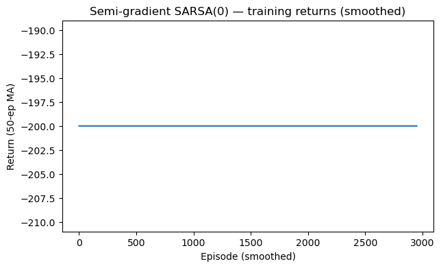
Figure 2.6: Average return w.r.t. episode (Semi-Gradient SARSA)

Figure 2.7: Example rollout (Semi-Gradient SARSA)

Semi-Gradient SARSA with Experience Replay. Inspired by the technique of experience replay (ER) popularized by DQN (see 2.2.4.2), we incorporated ER into semi-gradient SARSA, which breaks its on-policy nature. Fig. 2.8 displays the learning curve, which shows steady increase of the per-episode return. Applying the final learned policy to the mountain car yields a successful trajectory to the top of the mountain.

You can find code for the semi-gradient SARSA with experience replay algorithm here.

Figure 2.8: Average return w.r.t. episode (Semi-Gradient SARSA + Experience Replay)

Figure 2.9: Example rollout (Semi-Gradient SARSA + Experience Replay)

2.2.4 Off-Policy Control

Off-policy control seeks to learn the optimal action–value function while collecting data under a different behavior policy (e.g., an \(\varepsilon\)-soft policy). As in the tabular setting, Q-learning is the canonical off-policy control method. With function approximation, however, off-policy control becomes substantially harder than in the tabular case.

To illustrate why, we first present off-policy semi-gradient TD(0) for policy evaluation and use Baird’s counterexample (Baird et al. 1995) to highlight the deadly triad: bootstrapping + function approximation + off-policy sampling can cause divergence.

We then turn to the Deep Q-Network (DQN) (Mnih et al. 2015), which stabilizes Q-learning with two key mechanisms—experience replay and a target network—leading to landmark Atari results. Finally, we connect DQN to fitted Q-iteration (FQI) (Riedmiller 2005), a batch method with theoretical guarantees, to clarify why these stabilizations work (Fan et al. 2020).

2.2.4.1 Off-Policy Semi-Gradient TD(0)

Setup. We aim to estimate the state-value function of a target policy \(\pi\) using a different behavior policy \(b\). Since the state space is continuous, we employ function approximation to represent the value function as \(V(s;\theta)\) with \(\theta \in \mathbb{R}^d\). In the case of linear approximation, we have \(V(s;\theta) = \theta^\top \phi(s)\) where \(\phi(s)\) is a function that featurizes the state.

Semi-Gradient TD(0). Given a transition \((s_t,a_t,r_t,s_{t+1})\) collected under the behavior policy \(b\), form the TD error \[ \delta_t = r_t + \gamma V(s_{t+1}; \theta) - V(s_t;\theta). \] The off-policy Semi-Gradient TD(0) update reads \[\begin{equation} \theta \quad \leftarrow \quad \theta + \alpha_t \rho_t \delta_t \nabla_\theta V(s_t; \theta), \tag{2.59} \end{equation}\] where \(\rho_t\) is the likelihood ratio as in (2.37): \[ \rho_t = \frac{\pi(a_t \mid s_t)}{b(a_t \mid s_t)}. \] This off-policy semi-gradient TD(0) update (2.59) looks perfectly reasonable. However, the following Baird’s counterexample illustrates the instability of the algorithm.

Baird’s Counterexample. Consider an MDP with 7 states containing 6 upper states and 1 lower state, as shown in Fig. 2.10 (the figure comes from (Sutton and Barto 1998)). There are two actions, one called “solid” and the other called “dashed”. If the agent picks “solid” at any state, then the system transitons to the lower state with probability 1. If the agent picks “dashed” at any state, then the system transitions to any one of the upper states with equal probability. All rewards are zero, and the discount factor is \(\gamma=0.99\).

The target policy \(\pi\) always picks “solid”, while the behavior policy \(b\) picks “solid” with probability \(1/7\) and “dashed” with probability \(6/7\).

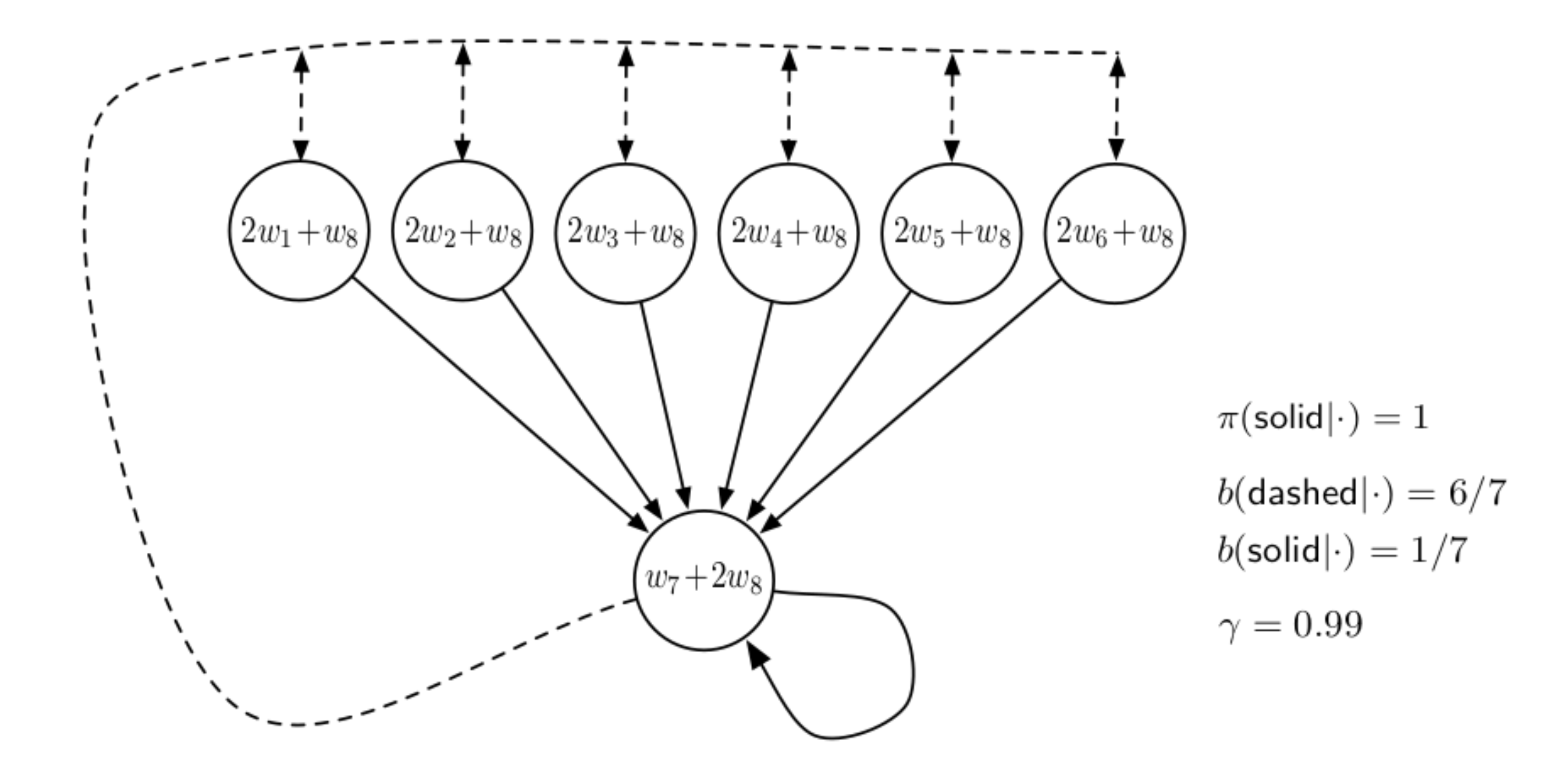
Figure 2.10: Baird Counterexample

Consider the case of linear function approximation where \(V(s;w) = w^\top \phi(s)\) where \(w \in \mathbb{R}^8\). For the upper states, the feature \(\phi(s)\) leads to \(V(s;w) = 2 w_1 + w_8\), and for the lower state, the feature \(\phi(s)\) leads to \(V(s;w) = w_7 + 2w_8\).

This Python script implements the off-policy semi-gradient TD(0) algorithm with importance sampling for policy evaluation.

Fig. 2.11 plots \(\Vert w \Vert_2\), the magnitude of \(w\), with respect to iterations. Clearly, we see the parameter \(w\) diverges under the off-policy semi-gradient TD(0) algorithm.

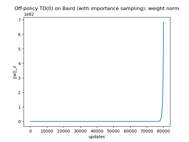
Figure 2.11: Baird Counterexample: divergence

The Deadly Triad. Three ingredients were used together in Baird’s example:

• Off-policy: a different behavior policy \(b\) is used to collect data for the evaluation of the target policy \(\pi\);

• Function approximation: the value function employs function approximation;

• Bootstrapping: the TD error uses the bootstrapped target “\(r_t + \gamma V(s_{t+1}; \theta)\)” instead of the full return as in Monte Carlo.

The “deadly triad” is used to illustrate that using all three ingredients together will lead to the potential divergence of policy evaluation.

Why? Recall that, using linear approximation, the on-policy Semi-Gradient TD(0) algorithm guarantees convergence to the unique fixed point of the projected Bellman equation (PBE) (2.54), restated here \[ V^\star_{\text{TD}} = \Pi_{\mu} T^\pi V^\star_{\text{TD}}, \] where \(\mu\) is the stationary distribution induced by the policy \(\pi\). A central reason for the guaranteed convergence is that the projected Bellman operator \[ \Pi_{\mu} T^\pi \] is a \(\gamma\)-contraction and has a unique fixed point. Therefore, the on-policy Semi-Gradient TD(0) algorithm—can be seen as a stochastic approximation of the projected Bellman operator—enjoys convergence guarantees.

However, in the off-policy case, the orthogonal projection \(\Pi_\mu\) needs to be modified as \(\Pi_{\nu}\), where \(\nu\) is the stationary distribution induced by the behavior policy \(b\). The new operator \[ \Pi_{\nu} T^\pi \] is not guaranteed to be a \(\gamma\)-contraction, due to the mismatch between \(\nu\)—induced by \(b\)—and the target policy \(\pi\). Therefore, divergence can potentially happen.

How to Fix? Multiple algorithms have been proposed to fix the deadly triad. Notable examples include the gradient TD (GTD) family of algorithms (Sutton, Szepesvári, and Maei 2008), (Sutton et al. 2009), and the Emphatic TD (ETD) learning algorithm (Mahmood et al. 2015). They are influential and widely cited, but they are not (yet) mainstream in deep RL practice. Their main appeal is theoretical—they provide off-policy evaluation algorithms with convergence guarantees under linear function approximation. Moreover, GTD/TDC require two-time-scale step-sizes and ETD’s emphatic weights can have high variance, making them less attractive for large-scale control with neural networks. I encourage you to read the papers to understand the algorithms. However, in the next, I will explain the deep Q network (DQN) approach that is more popular in practice.

2.2.4.2 Deep Q Network

We consider continuous state spaces with a finite action set, and a parametric action–value function \(Q(s,a; \theta)\).

Naive (semi-gradient) Q-Learning with Function Approximation. The goal is to learn \(Q^\star\) and act \(\varepsilon\)-greedily w.r.t. \(Q(\cdot,\cdot; \theta)\). The update uses a bootstrapped optimality target built from the current network. \[\begin{equation} \begin{split} y_t & = r_t + \gamma \max_{a'} Q(s_{t+1}, a';\theta) \\ \theta & \leftarrow \theta + \alpha \,\big(y_t - Q(s_t,a_t;\theta)\big)\,\nabla_\theta Q(s_t,a_t; \theta). \end{split} \tag{2.60} \end{equation}\] The transitions \((s_t,a_t,r_t,s_{t+1})\) are generated using a \(\varepsilon\)-greedy policy with respect to \(Q(s,a;\theta)\).

This naive variant is off-policy + bootstrapping + function approximation (i.e., the deadly triad) and thus can be unstable.

Deep Q Network (DQN) with Experience Replay (ER) and Target Network (TN). DQN augments the above naive Q learning with two stabilizers:

• Experience Replay (ER): store transitions in a buffer \(\mathcal{D}\); train on i.i.d.-like mini-batches to decorrelate updates and reuse data.

• Target Network (TN): maintain a delayed copy \(Q(\cdot,\cdot; \theta^-)\) to compute targets \[ y_t = r_t + \gamma \max_{a'} Q(s_{t+1},a';\theta^-), \] keeping the target fixed for many gradient steps.

The full DQN algorithm is presented below.

• Initialize replay buffer \(\mathcal{D}\) with capacity \(N\)
• Initialize approximate Q value \(Q(s,a;\theta)\)
• Initialize target \(Q_T(s,a;\theta^-)\) with \(\theta^- = \theta\)
• For episode \(=1,\dots,M\) do:
  • Initialize \(s_0\)
  • For \(t=0,\dots,T\) do:
    • \(\varepsilon\)-greedy policy:
      • With probability \(\varepsilon\) select a random action \(a_t \in \mathcal{A}\)
      • Otherwise select \(a_t = \arg\max_a Q(s_t,a_t;\theta)\)
    • Observe transition \(\tau_t = (s_t, a_t, r_t, s_{t+1})\)
    • Put \(\tau_t\) inside replay buffer \(\mathcal{D}\)
    • Sample a random minibatch of transitions \(\{(s_i, a_i, r_i, s_{i+1})\}_{i \in \mathcal{I}}\) from \(\mathcal{D}\)
    • For \(i \in \mathcal{I}\) do:
      • Set target \(y_i = r_i + \gamma \max_a Q_T(s_{i+1}, a; \theta^-)\) using the target network
      • Update \(\theta \leftarrow \theta + \alpha (y_i - Q(s_i,a_i;\theta)) \nabla_\theta Q(s_i, a_i; \theta)\)
    • Every \(C\) steps synchronize the target network with the \(Q\) net: \(\theta^- = \theta\)

Although the naive Q-leanring with function approximation can be unstable, DQN has achieved great success and is also very efficient (Mnih et al. 2015).

Fitted Q Iteration (FQI). To understand why DQN can achieve stabilized training compared to naive Q-learning with function approximation. It is insightful to look at the fitted Q iteration (FQI) algorithm, presented below.

• Initialize \(Q^{(0)} = Q(s,a;\theta_0)\)
• For \(k=0,1,2,\dots,K-1\) do:
  • Sample i.i.d. transitions \(\{ (s_i,a_i,r_i,s_{i+1}) \}_{i=1}^N\) with \((s_i, a_i)\) drawn from a distribution \(\mu\)
  • Compute targets \(y_i = r_i + \gamma \max_a Q^{(k)}(s_{t+1},a;\theta_k),i=1,\dots,N\)
  • Update the action-value function: \[ Q^{(k+1)} = Q(s,a;\theta_{k+1}), \quad \theta_{k+1} \in \arg\min_{\theta} \frac{1}{N} \sum_{i=1}^N (y_i - Q(s_i,a_i;\theta))^2 \]

The FQI algorithm samples trajectories from a fixed distribution \(\mu\) and optimizes the parameter using targets generated from those trajectories. Under reasonable coverage and approximation assumptions, it converges and admits finite-sample error bounds (Antos, Szepesvári, and Munos 2007), (Munos and Szepesvári 2008).

Connection to DQN. DQN is similar to FQI in the following aspects.

• Frozen targets: DQN’s target network \(Q(\cdot,\cdot; \theta^-)\) plays the role of \(Q^{(k-1)}\) in FQI.

• Supervised fit: DQN’s mini-batch loss minimizes \(\sum (Q(s_i,a_i; \theta) - y_i)^2\), just like FQI’s regression step.

• Data usage: FQI trains on a fixed dataset; DQN’s replay buffer approximates training on an (ever-growing) quasi-fixed dataset by repeatedly sampling past transitions.

• Iteration vs. updates: FQI alternates full regressions and target recomputation; DQN alternates many SGD steps with periodic target updates. In the limit of many SGD steps per target update and a large replay buffer, DQN \(\approx\) online, incremental FQI.

This perspective explains why ER + TN make DQN far more stable than naive Q-learning with function approximation: they make the optimization behave like a sequence of supervised fits to fixed targets drawn from a nearly stationary dataset.

Example 2.4 (DQN for Mountain Car) Consider again the Mountain car problem from Example 2.3.

Naive Q-Learning with Function Approximation. As shown in Fig. 2.12 and Fig. 2.13, naive Q-leanring with function approximation fails to learn a good policy.

Figure 2.12: Average return w.r.t. episode (Naive Q Learning)

Figure 2.13: Example rollout (Naive Q Learning)

DQN with Experience Replay and Target Network. Adding ER and TN to Q-learning leads to steady learning (Fig. 2.14) and a successful final policy (Fig. 2.15).

You can find code for these experiments here.

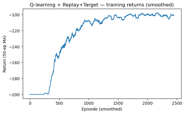
Figure 2.14: Average return w.r.t. episode (DQN)

Figure 2.15: Example rollout (DQN)

References

Antos, András, Csaba Szepesvári, and Rémi Munos. 2007. “Fitted q-Iteration in Continuous Action-Space MDPs.” Advances in Neural Information Processing Systems 20.

Baird, Leemon et al. 1995. “Residual Algorithms: Reinforcement Learning with Function Approximation.” In Proceedings of the Twelfth International Conference on Machine Learning, 30–37.

Fan, Jianqing, Zhaoran Wang, Yuchen Xie, and Zhuoran Yang. 2020. “A Theoretical Analysis of Deep q-Learning.” In Learning for Dynamics and Control, 486–89. PMLR.

Kearns, Michael J, and Satinder Singh. 2000. “Bias-Variance Error Bounds for Temporal Difference Updates.” In COLT, 142–47.

Mahmood, A Rupam, Huizhen Yu, Martha White, and Richard S Sutton. 2015. “Emphatic Temporal-Difference Learning.” arXiv Preprint arXiv:1507.01569.

Mnih, Volodymyr, Koray Kavukcuoglu, David Silver, Andrei A Rusu, Joel Veness, Marc G Bellemare, Alex Graves, et al. 2015. “Human-Level Control Through Deep Reinforcement Learning.” Nature 518 (7540): 529–33.

Munos, Rémi, and Csaba Szepesvári. 2008. “Finite-Time Bounds for Fitted Value Iteration.” Journal of Machine Learning Research 9 (5).

Riedmiller, Martin. 2005. “Neural Fitted q Iteration–First Experiences with a Data Efficient Neural Reinforcement Learning Method.” In European Conference on Machine Learning, 317–28. Springer.

Robbins, Herbert, and David Siegmund. 1971. “A Convergence Theorem for Non Negative Almost Supermartingales and Some Applications.” In Optimizing Methods in Statistics, 233–57. Elsevier.

Sutton, Richard S, and Andrew G Barto. 1998. Reinforcement Learning: An Introduction. Vol. 1. 1. MIT press Cambridge.

Sutton, Richard S, Hamid Reza Maei, Doina Precup, Shalabh Bhatnagar, David Silver, Csaba Szepesvári, and Eric Wiewiora. 2009. “Fast Gradient-Descent Methods for Temporal-Difference Learning with Linear Function Approximation.” In Proceedings of the 26th Annual International Conference on Machine Learning, 993–1000.

Sutton, Richard S, Csaba Szepesvári, and Hamid Reza Maei. 2008. “A Convergent o(n) Algorithm for Off-Policy Temporal-Difference Learning with Linear Function Approximation.” Advances in Neural Information Processing Systems 21 (21): 1609–16.