Chapter 3 Approximate Optimal Control

Thanks to Jiarui Li for contributing to this Chapter.

In Chapter 2, we have studied two cases where dynamic programming (DP) can be executed exactly. Both cases are interesting yet limiting.

In the linear quadratic regulator (LQR) case, the optimal controller is a linear controller and it does not require discretization of the state and control space. However, LQR only handles systems with linear dynamics.

In the Markov Decision Process (MDP) case, value iteration can obtain the optimal cost-to-go (or the optimal \(Q\)-value function) usually in a finite number of iterations. With barycentric interpolation, value iteration also leads to a practical controller for swinging up the pendulum (see Example 2.3), at least starting from some initial states. However, value iteration suffers from the curse of dimensionality, i.e., the amount of memory and computation needed to compute the optimal cost-to-go grows exponentially with the number of grids used to discretize the state space and control space.

In this Chapter, we will study approximate dynamic programming, which aims to not find the optimal controller (simply because it is too demanding), but only a suboptimal controller that is perhaps good enough. It is worth noting that there exists a large amount of algorithms and literature for approximate DP, most of which are closely related to reinforcement learning, and studying all of them is beyond the scope of this course. In the following we will only go through several algorithmic frameworks that are representative.

3.1 Fitted Value Iteration

Let us consider the infinite-horizon optimal control problem introduced in Chapter 1.3 \[ \min_{\pi} \mathbb{E} \left\{ \sum_{k=0}^\infty g(x_k, \pi(x_k)) \right\}. \] Under some technical conditions, we know that the optimal policy is a deterministic and stationary policy and the optimal cost-to-go satisfies the following Bellman Optimality Equation \[\begin{equation} J^\star(x) = \min_{u \in \mathbb{U}} \mathbb{E}_w \left\{ g(x,u) + J^\star(f(x,u,w)) \right\}, \quad \forall x \in \mathbb{X}. \tag{3.1} \end{equation}\] From the plots in Example 2.3, we observe that even for a “simple” problem like pendulum swing-up, the optimal cost-to-go \(J^\star(x)\) does not look simple at all.

So here comes a very natural idea. What if we parametrize a cost-to-go function \(\tilde{J}(x,r)\) by a vector of unknown coefficients \(r \in \mathbb{R}^{d}\) and ask \(\tilde{J}(x,r)\) to satisfy (3.1) as closely as possible?

This indeed leads to a valid algoithm called fitted value iteration (FVI).

In FVI, we initialize the parameters \(r\) as \(r_0\) in the first step. Then, at the \(k\)-th iteration, we perform two subroutines.

Value update. Firstly, we sample a large amount of points in the state space \(\{x_k^s \}_{s=1}^q\), and for each \(x_k^s\), we solve the minimization problem on the right-hand side of (3.1) using \(J(x,r^{(k)})\) as the cost-to-go. Formally, this is \[\begin{equation} \beta_k^s \leftarrow \min_{u \in \mathbb{U}} \mathbb{E}_w \left\{ g(x_k^s, u) + \tilde{J}(f(x_k^s,u,w),r^{(k)}) \right\}, \quad \forall x_k^s, s= 1,\dots,q. \tag{3.2} \end{equation}\] This step gives us a list of scalars \(\{ \beta_k^s \}_{s=1}^q\). If \(\tilde{J}(x,r)\) indeed satisfies the Bellman optimality equation, then we should have \[ \tilde{J}(x_k^s,r^{(k)}) = \beta_k^s, \quad \forall s = 1,\dots,q. \] This is certainly not true when the parameter \(r\) is imperfect.

Parameter update. Therefore, we will see the best parameter that minimizes the violation of the above equation \[\begin{equation} r^{(k+1)} \leftarrow \arg\min_{r \in \mathbb{R}^d} \sum_{s=1}^q \left(\tilde{J}(x_k^s,r) - \beta_k^s\right)^2. \tag{3.3} \end{equation}\] FVI essentially carries out (3.2) and (3.3) until some convergence metric is met.

Two challenges immediately show up:

• How to perform the minimization over \(u\) in the first step (3.2)?

• How to find the best parameter update in the second step (3.3)?

To solve the first challenge, we will assume that \(\mathbb{U}\) is a finite set so that minimization over \(u\) can be solved exactly. Note that this assumption is not strictly necessary. In fact, as long as \(\mathbb{U}\) is a convex set and the objective in (3.2) is also convex, then the minimization can also be solved exactly (A. Yang and Boyd 2023). However, we assume \(\mathbb{U}\) is finite to simplify our presentation.

To solve the second challenge, we will assume \(\tilde{J}(x,r)\) is linear in the parameters \(r\), as we will study further in the following.

3.1.1 Linear Features

We parameterize \(\tilde{J}(x,r)\) as follows: \[\begin{equation} \tilde{J}(x,r) = \sum_{i=1}^d r_i \cdot \phi_i(x) = \begin{bmatrix} \phi_1(x) & \cdots & \phi_d(x) \end{bmatrix} r = \phi(x)^T r, \end{equation}\] where \(\phi_1(x),\dots,\phi_d(x)\) are a set of known basis functions, or features. Common examples of features include polynomials and radial basis functions. With this parametrization, the optimization in (3.3) becomes \[\begin{equation} \min_{r \in \mathbb{R}^d} \sum_{s=1}^q \left( \phi(x_k^s)^T r - \beta_k^s \right)^2, \tag{3.4} \end{equation}\] which is a least-squares problem that can be solved in closed form. In particular, we can compute the gradient of its objective with respect to \(r\) and set it to zero, leading to \[\begin{align} 0 = \sum_{s=1}^q 2(\phi(x_k^s)^T r - \beta_k^s ) \phi(x_k^s) \Longrightarrow \\ r = \left( \sum_{s=1}^q \phi(x_k^s) \phi(x_k^s)^T \right)^{-1} \left( \sum_{s=1}^q \beta_k^s \phi(x_k^s) \right). \end{align}\]

Let us apply FVI with linear features to a linear system for which we know the optimal cost-to-go.

Example 3.1 (Fitted Value Iteration for Double Integrator) Consider the double integrator \[ \ddot{q} = u. \] Take \(x = [q;\dot{q}]\), we can write the dynamics in state-space form \[\begin{equation} \dot{x} = \begin{bmatrix} \dot{q} \\ u \end{bmatrix} = \begin{bmatrix} 0 & 1 \\ 0 & 0 \end{bmatrix} x + \begin{bmatrix} 0 \\ 1 \end{bmatrix} u \tag{3.5} \end{equation}\] We use a constant time \(h=0.01\) differentiation to convert the continuous-time dynamics into discrete-time: \[ x_{k+1} = h \cdot \dot{x}_k + x_k = \begin{bmatrix} 1 & h \\ 0 & 1 \end{bmatrix} x_k + \begin{bmatrix} 0 \\ h \end{bmatrix} u_k. \]

The goal is to regulate the system at \((0,0)\). To do so, we use a quadratic cost \[ J(x) = \min \sum_{k=0}^{\infty} x_k^T Q x_k + u_k^T R u_k, \quad x_0 = x. \] with \(Q = 0.1I_2\) and \(R = 1\).

In Chapter 2, we learned how to use LQR to precisely calculate the cost-to-go function of these systems using the Algebraic Recatti Equation. Solving the ARE, we obtain \[ S_{\mathrm{LQR}} = \begin{bmatrix} 27.1640 & 31.7584 \\ 31.7584 & 85.9510 \end{bmatrix}. \]

Now we want to investigate if FVI can find the same matrix \(S\). To do so, we parametrize \[ \tilde{J}(x) = x^T S x = x^T \begin{bmatrix} S_1 & S_2 \\ S_2 & S_3 \end{bmatrix} x = \begin{bmatrix} x_1^2 & 2 x_1 x_2 & x_2^2 \end{bmatrix} \begin{bmatrix} S_1 \\ S_2 \\ S_3 \end{bmatrix}, \] where \(S\) only has three independent variables due to being symmetric. Do note that \(\tilde{J}(x)\) is linear in \(S\), so the parameter update step can be solved in closed form.

We now show that the value update step can also be solved in closed form. Suppose we choose \(x_k\) as a sample, then the right-hand side of (3.2) reads: \[ \min_{u} x_k^T Q x_k + u^2 + (A x_k + B u)^T S^{(k)} (A x_k + B u), \] where \(S^{(k)}\) is the value of \(S\) at the \(k\)-th iteration. Clearly, the optimization problem above is a convex quadratic optimization and can be solved in closed form: \[ u = - (1 + B^T S^{(k)} B) ^{-1} B^T S^{(k)} A x_k. \]

Applying fitted value iteration on randomly sampled points mentioned above, we obtain the fitted \(S\) \[ S_{\mathrm{FVI}} = \begin{bmatrix} 27.1640 & 31.7583 \\ 31.7584 & 85.9509 \end{bmatrix}. \]

We can see that \(S_{\mathrm{FVI}}\) almost exactly matches the groundtruth LQR solution \(S_{\mathrm{LQR}}\).

You can play with the code here.

3.1.2 Neural Network Features

We have seen that simple quadratic features work for the LQR problem. For more complicated problems, we will need more powerful function approximators like neural networks.

When we parameterize \(\tilde{J}(x,r)\) as a neural network, \(r\) will be the weights of the neural network. We may still be able to solve the value update step if \(u\) lives in a finite space. However, the parameter update step usually cannot be solved exactly and will need to rely on numerical algoithms such as gradient descent.

Let us try neural FVI on the same double integrator problem.

Example 3.2 (Neural Fitted Value Iteration for the Double Integrator) In this example, we will use neural network as the approximation of the cost-to-go function and conduct neural FVI on a double integrator. The dynamics of the double integrator has been introduced in example 3.1. We use a positive definite network to model the cost-to-go function \[\begin{equation} J(x) = N(x)^T N(x), \end{equation}\] where \(N(x)\) is a 3-layer Multi-Layer-Perceptron with ReLU activation.

Using mini-batch learning plus Adam optimizer, we obtain the cost-to-go in Fig. 3.1 after 300 epochs of training.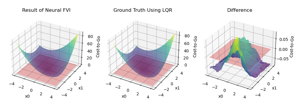

Figure 3.1: Comparison between the result of NN-based FVI and ground truth

The figure shows that the approximation performance of NN is pretty good. Simulation experiments also shows that the corresponding controller could successfully regulate the system at \((0,0)\).

You can see the code here.

3.1.3 Fitted Q-value Iteration

From the MDP Chapter we know there is an equivalent representation of the Bellman Optimality Equation by replacing the \(J\) value function in (3.1) with the \(Q\)-value function \(Q(x,u)\). In particular, with \[ J^\star(x) = \min_{u \in \mathbb{U}} Q^\star(x,u) \] substituted into (3.1), we obtain the Bellman Optimality Equation in \(Q^\star(x,u)\): \[\begin{equation} Q^\star(x,u) = g(x,u) + \mathbb{E}_w \left\{ \min_{u' \in \mathbb{U}} Q^\star(f(x,u,w),u') \right\}. \tag{3.6} \end{equation}\] We can then use the same idea to approximate \(Q^\star(x,u)\) as \[ \tilde{Q}(x,u,r) \] with \(r \in \mathbb{R}^d\) a parameter vector. By iteratively evaluating the right-hand side of (3.6), we obtain the algoithm known as fitted \(Q\)-value iteration (FQI).

For example, we can similarly adopt the linear feature parameterization and set \[ \tilde{Q}(x,u,r) = \phi(x,u)^T r, \] where \(\phi(x,u)\) is a known pre-selected feature vector. Then at the \(k\)-th iteration of FQI, we perform two subroutines.

Value update. We sample a number of state-control pairs \(\{(x_k^s,u_k^s) \}_{s=1}^q\) and evaluate the right-hand side of the Bellman optimality equation (3.6): \[\begin{equation} \beta_k^s \leftarrow g(x_k^s,u_k^s) + \mathbb{E}_w \left\{ \min_{u' \in \mathbb{U}} \tilde{Q}(f(x_k^s,u_k^s,w),u',r^{(k)}) \right\}, \quad \forall s = 1,\dots,q. \tag{3.7} \end{equation}\] Again, if \(u\) lives in a finite space, or the minimization is convex, the above value update can be solved exactly.

Parameter update. We update the parameter vector using the updated values \(\{ \beta_k^s \}_{s=1}^q\): \[\begin{equation} r^{(k+1)} \leftarrow \arg\min_{r \in \mathbb{R}^d} \sum_{s=1}^q \left( \tilde{Q}(x_k^s,u_k^s,r) - \beta_k^s \right)^2, \tag{3.8} \end{equation}\] which is a least squares problem that can be solved in closed form.

Let us apply FQI to the same double integrator example.

Example 3.3 (Fitted Q-value Iteration for Double Integrator) Consider the same double integrator dynamics in Example 3.1.

From the LQR solution we know the optimal \(Q\)-value function is \[\begin{align} Q^\star(x,u) &= x^T Q x + u^T R u + (Ax + Bu)^T S (Ax + Bu) \\ &= \begin{bmatrix} x \\ u \end{bmatrix}^T \underbrace{\begin{bmatrix} A^T S A + Q & A^T S B \\ B^T S A & B^T S B + R \end{bmatrix}}_{M_{\mathrm{LQR}}} \begin{bmatrix} x \\ u \end{bmatrix}, \end{align}\] where \(M_{\mathrm{LQR}}\) is \[ M_{\mathrm{LQR}} = \begin{bmatrix} 27.2640 & 32.0300 & 0.3176 \\ 32.0300 & 86.6889 & 0.8627 \\ 0.3176 & 0.8627 & 1.0086 \end{bmatrix}. \]

Let us apply FQI to see if we get the same solution. We parametrize \[\begin{align} \tilde{Q}(x,u) &= \begin{bmatrix} x \\ u \end{bmatrix}^T \begin{bmatrix} M_1 & M_2 & M_3 \\ M_2 & M_4 & M_5 \\ M_3 & M_5 & M_6 \end{bmatrix} \begin{bmatrix} x \\ u \end{bmatrix} \\ &= \begin{bmatrix} x_1^2 & 2 x_1 x_2 & 2x_1 u & x_2^2 & 2x_2 u & u^2 \end{bmatrix} \begin{bmatrix} M_1 \\ M_2 \\ M_3 \\ M_4 \\ M_5 \\ M_6 \end{bmatrix}. \end{align}\]

At the \(k\)-th FQI iteration, we are given \(M^{(k)}\). Suppose we sample \((x_k, u_k)\), then the value update step needs to solve (3.7), which reads: \[ \beta_k = g(x_k, u_k) + \min_{u'} \underbrace{\begin{bmatrix} A x_k + B u_k \\ u' \end{bmatrix}^T M^{(k)} \begin{bmatrix} A x_k + B u_k \\ u' \end{bmatrix}}_{\psi(u')}. \] The objective function \(\psi(u')\) can be shown to be quadratic: \[ \psi(u') = (Lu' + a_k)^T M^{(k)} (Lu' + a_k), \quad L = \begin{bmatrix} 0 \\ 1 \end{bmatrix}, a_k = \begin{bmatrix} A x_k + B u_k \\ 0 \end{bmatrix}. \] Therefore, we can solve \(u'\) in closed-form \[ u' = - (L^T M^{(k)} L)^{-1} L^T M^{(k)} a_k. \]

Applying FQI with the closed-form update above, we get \[ M_{\mathrm{FQI}} = \begin{bmatrix} 27.2640 & 32.0300 & 0.3176 \\ 32.0300 & 86.6889 & 0.8627 \\ 0.3176 & 0.8627 & 1.0086 \end{bmatrix}, \] which is exactly the same as the solution obtained from LQR.

You can play with the code here.

3.1.4 Deep Q Network

Although we have only tested FVI and FQI on the simple double integrator linear system, these algoithms are really not so different from the state-of-the-art reinforcement learning algoithms. For example, the core of the seminal work Deep \(Q\)-Network (DQN) (Mnih et al. 2015) is to use a deep neural network to parameterize the \(Q\)-value function. Of course the DQN work has used other clever ideas to make it work in practice, such as experience replay, but the essence is fitted \(Q\)-value iteration.

You can find a good explanation of DQN in this tutorial, and a practical step-by-step Pytorch implementation that applies DQN on the cart-pole system.

3.1.5 Deep + Shallow

Combine the rich features of DQN with the stable learning of FQI (Levine et al. 2017).

3.2 Trajectory Optimization

Consider a continuous-time optimal control problem (OCP) in full generality \[\begin{equation} \begin{split} \min_{u(t), t \in [0,T]} & \quad g_T(x(T)) + \int_{t = 0}^T g(x(t),u(t)) dt \\ \text{subject to} & \quad \dot{x} = f(x(t),u(t)) \\ & \quad x(0) = x_0 \\ & \quad (x(t),u(t)) \in \mathcal{X} \times \mathcal{U} \\ & \quad \phi_i (x(t),u(t)) \geq 0, i=1,\dots,q. \end{split} \tag{3.9} \end{equation}\] where \(g_T\) the terminal cost, \(g\) the running cost, \(x_0\) the initial condition, \(\mathcal{X}\) the state constraint set, \(\mathcal{U}\) the control constraint set, and \(\{ \phi_i \}_{i=1}^q\) are general state-control constraints. We assume that the state constraint set \(\mathcal{X}\) and control constraint set \(\mathcal{U}\) can be described by a finite set of inequalities, i.e., \[ \mathcal{X} = \{x \in \mathbb{R}^n \mid c^x_i(x) \geq 0, i =1,\dots,q_x\}, \quad \mathcal{U} = \{u \in \mathbb{R}^m \mid c^u_i(u) \geq 0, i = 1,\dots,q_u \}. \] Assume that all functions are differentiable.

Our goal is to “transcribe” the infinite-dimensional continuous-time optimization (3.9) into a nonlinear programming problem (NLP) of the following form \[\begin{equation} \begin{split} \min_{v \in \mathbb{R}^{n_v}} & \quad c(v) \\ \text{subject to} & \quad c_{\text{eq},i}(v) = 0, i =1,\dots, n_{\text{eq}} \\ & \quad c_{\text{ineq},i}(v) \geq 0, i=1,\dots,n_{\text{ineq}}, \end{split} \tag{3.10} \end{equation}\] where \(v\) is a finite-dimensional vector variable to be optimized, \(c, c_{\text{eq},i}, c_{\text{ineq},i}\) are (continuously differentiable) objective and constraint functions. Once we have done the transcription from (3.9) to (3.10), then we have a good number of numerical optimization algorithms at our disposal. For example, the Matlab fmincon provides a nice interface to many such algorithms, e.g., interior-point method and sequential quadratic programming. You have already played with a simple example of fmincon in Exercise 9.1. Other well-implemented NLP algorithms include IPOPT and SNOPT. However, usually the Matlab fmincon gives a decent start point for trying out different algorithms before moving to commercial solvers such as SNOPT. For a more comprehensive understanding about how NLP algoithms work under the hood, I suggest reading (Nocedal and Wright 1999).

Before we talk about how to transcribe the OCP into an NLP, let us use a simple example to get a taste of fmincon.

Example 3.4 (Fire a Canon with fmincon) On a 2D plane, suppose we have a canon at the origin \((0,0)\), and we want to fire the canon, with control over the initial velocity \((v_1, v_2)\), so that the canon ball hits the target location \((10,10)\).

From our basic physics knowledge, we know the trajectory of the canon ball is described by \[ \begin{cases} x_1(t) = v_1 t \\ x_2(t) = v_2 t - \frac{1}{2}g t^2, \end{cases} \] where \(g\) is the gravity constant.

With the trajectory of the canon ball written above, we can formulate our nonlinear programming problem (NLP) as: \[\begin{equation} \begin{split} \min_{v_1, v_2, T} & \quad \frac{1}{2} (v_1^2 + v_2^2) \\ \text{subject to} & \quad v_1, v_2, T \geq 0 \\ & \quad x_1(T) = v_1 T = 10 \\ & \quad x_2(T) = v_2 T - \frac{1}{2}g T^2 = 10 \end{split} \tag{3.11} \end{equation}\] where our unknown variables are the initial velocities and the time \(T\) at which the canon ball hits the target. In the NLP (3.11), the first constraint asks all our varaibles to be nonnegative, the second and third constraints enforce the canon ball to hit the target.

The following script formulates the NLP (3.11) in matlab.

clc; clear; close all;
g = 9.8;
x0 = [0;0;1]; % initial guess of the solution
% define objective function
obj = @(x) objective(x);
% define nonlinear constraints
nonlincon = @(x) nonlinear_con(x,g);
% define options for fmincon
options = optimoptions('fmincon','Algorithm','interior-point',...
    'SpecifyObjectiveGradient',true,'SpecifyConstraintGradient',true,...
    'checkGradients',false);
% call fmincon
[xopt,fopt,~,out] = fmincon(obj,x0,... % objective and initial guess
    -eye(3),zeros(3,1),... % linear inequality constraints
    [],[],... % no linear equality constraints
    [],[],... % no upper and lower bounds
    nonlincon,... % nonlinear constraints
    options);
fprintf("Maximum constraint violation: %3.2f.\n",out.constrviolation);
fprintf("Objective: %3.2f.\n",fopt);
% plot the solution
T = xopt(3);
t = 0:0.01:T;
xt = xopt(1)*t;
yt = xopt(2)*t - 0.5*g*(t.^2);
figure;
plot(xt,yt,'LineWidth',2);
hold on
scatter(10,10,100,"red",'filled','diamond');
axis equal; grid on;
xlabel('$x_1(t)$','FontSize',24,'Interpreter','latex');
ylabel('$x_2(t)$','FontSize',24,'Interpreter','latex');
ax = gca; ax.FontSize = 20;
%% helper functions
function [f,df] = objective(x)
% x is our decision variable: [v1, v2, T]
% objective function
f = 0.5 * (x(1)^2 + x(2)^2);
% gradient of the objective function (optional)
df = [x(1); x(2); 0]; % column vector
end

function [c,ceq,dc,dceq] = nonlinear_con(x,g)
% no inequality constraints
c = []; dc = [];
% two equality constraints
ceq = [x(1)*x(3)-10;
       x(2)*x(3)-0.5*g*x(3)^2-10];
% explicit gradient of ceq
dceq = [x(3), 0;
        0, x(3);
        x(1), x(2)-g*x(3)];
end

Running the code above, we get the following trajectory

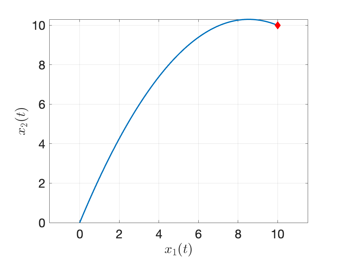
Figure 3.2: Trajectory of the canon ball obtained from fmincon.

What if you change the initial guess to fmincon, or add more constraints? Feel free to play with the code here.

It turns out there are multiple different ways to transcribe the optimal control problem (3.9) as the nonlinear programming problem (3.10). In the following, we will introduce three different formulations, direct single shooting, direct multiple shooting, and direct collocation.

3.2.1 Direct Single Shooting

In direct single shooting, we transcribe the OCP to the NLP by only optimizing a sequence of control values, with the intuition being that the state values are functions of the controls by invoking the system dynamics. In particular, we follow the procedure below.

Time discretization. We first discretize the total time window \([0,T]\) into a set of \(N\) intervals: \[ 0 = t_0 \leq t_1 \leq \dots \leq t_k \leq t_{k+1} \leq \dots \leq t_N = T. \] We denote \[ h_k = t_{k+1} - t_k \] as the length of the \(k\)-th time interval.

Piece-wise constant control. We will approximate the continuous-time control signal \(u(t)\) as a piece-wise constant function, i.e., \[ u(t) = u_k, \forall t \in [t_k, t_{k+1}). \] This is shown in Fig. 3.3. Let us collect all the constant control values as our decision variable to be optimized \[\begin{equation} v = \begin{bmatrix} u_0 \\ u_1 \\ \vdots \\ u_{N-1} \end{bmatrix} \in \mathbb{R}^{N m}. \tag{3.12} \end{equation}\] This \(v\) will be our variable in the NLP (3.10). Note that \(v\) has dimension \(N m\).

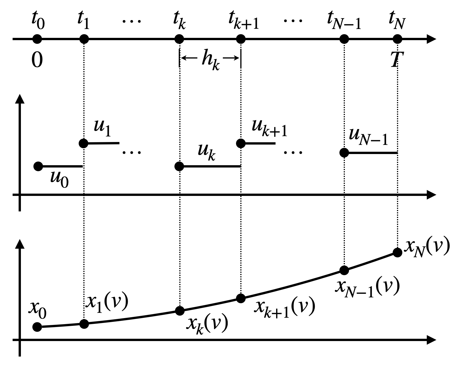
Figure 3.3: Direct single shooting.

Dynamics integration. It is clear that once \(v\) in (3.12), i.e., the set of controls, is determined, then the state trajectory \(x(t)\) is also uniquely determined by the initial condition \(x(0) = x_0\) and the dynamics \[ \dot{x}(t) = f(x(t),u(t)). \] In order to enforce the state constraint \(x(t) \in \mathcal{X}\), we will enforce the values of \(x\) at \(t_0,t_1,\dots,t_N\), i.e., \(x_k = x(t_k)\), to lie in the constraint set \(\mathcal{X}\). To do so, we need to integrate the dynamics. When the dynamics is linear, this integration can be done in closed form: \[ x_{k+1} = x_k + \int_{\tau=t_k}^{t_k + h_k} A x(\tau) + B u(\tau) d\tau = e^{Ah_k} x_k + A^{-1}(e^{Ah_k} - I) B u_k. \] By running the above equation from \(k=0\) to \(k=N-1\), we obtain the values of \(x_k,k=1,\dots,N\) as functions of the control vectors \(v\), shown in Fig. 3.3. When the dynamics is nonlinear, we will need to perform the dynamics integration using numerical integration. One of the most well known family of integrators is called “Runge-Kutta methods”. Among the family of methods, RK45 is perhaps the most popular one. We now briefly describe how a fourth-order RK integrator, i.e., RK4, works. Suppose we have already computed \(x_k\), and we want to integrate the dynamics to obtain \(x_{k+1}\). The RK4 integrator first computes the time derivatives at a sequence of four points: \[\begin{align} \alpha_1 &= f(x_k, u_k) \\ \alpha_2 &= f\left( x_k + \frac{1}{2} h_k \alpha_1, u_k \right) \\ \alpha_3 &= f\left( x_k + \frac{1}{2} h_k \alpha_2, u_k \right) \\ \alpha_4 &= f\left( x_k + h_k \alpha_3, u_k \right). \end{align}\] Then we can obtain \(x_{k+1}\) via a weighted sum of the \(\alpha_i\)’s \[\begin{equation} x_{k+1} = x_k + \frac{1}{6} h_k \left( \alpha_1 + 2 \alpha_2 + 2 \alpha_3 + \alpha_4 \right) = \text{RK4}(x_k, u_k). \tag{3.13} \end{equation}\] Notice that a naive integrator would just perform \(x_{k+1} = x_k + h_k \alpha_1\) without querying the gradients at three other points. The nice property of RK4 is that it leads to better accuracy than the naive integration. Writing the RK4 integrator recursively, we obtain \[ x_{k+1} = \text{RK4}(x_k, u_k) = \text{RK4}(\text{RK4}(x_{k-1},u_{k-1}),u_k) = \text{RK4}(\text{RK4}(...(x_0,u_0))...u_k), \] where RK4 is invoked for \(k+1\) times. Clearly, each \(x_k\) is a complicated function of the sequence of controls \(v\) and the initial state \(x_0\). We will write \(x_k(v)\) to make this explict, as shown in Fig. 3.3.

Objective approximation. We can approximate the objective of the OCP (3.9) using trapezoidal integration: \[ g_T(x(T)) + \int_{t=0}^T g(x(t),u(t)) dt \approx g_T(x_N(v)) + \sum_{k=0}^{N-1} \frac{h_k}{2}(g(x_k(v),u_k) + g(x_{k+1}(v),u_{k+1})). \]

Summary. In summary, the transcribed NLP for the optimal control problem using direct single shooting would be \[\begin{equation} \begin{split} \min_{v = (u_0,\dots,u_{N-1})} & \quad g_T(x_N(v)) + \sum_{k=0}^{N-1} \frac{g(x_k(v),u_k) + g(x_{k+1}(v), u_{k+1})}{2} h_k \\ \text{subject to} & \quad c^u_i(u_k) \geq 0, i=1,\dots,q_u, \quad k=0,\dots,N-1 \\ & \quad c^x_i(x_k(v)) \geq 0, i=1,\dots,q_x, \quad k=1,\dots,N \\ & \quad \phi_i(x_k(v),u_k) \geq 0, i=1,\dots, q, \quad k=0,\dots,N. \end{split} \tag{3.14} \end{equation}\]

Pros and Cons. The advantage of using direct single shooting to transcribe the OCP is clear: it leads to fewer variables because the only decision variables in (3.14) are the sequence of controls. In other transcription methods, the decision variable of the NLP typically involves the states as well. The disadvantage of direct single shooting is the complication of the function \(x_k(v)\) caused by numerical integrators such as RK4. Even though the original continuous-time dynamics \(f(x,u)\) may be simple, the RK4 function can be highly complicated due to evaluating \(\dot{x}\) at multiple other locations. Moreover, the recursion of the RK4 operator makes this complication even worse.

Let us try the RK4 simulator for a simple example.

Example 3.5 (Propagation of Nonlinearities) Consider the following dynamics \[ x = \begin{bmatrix} x_1 \\ x_2 \\ x_3 \end{bmatrix}, \quad \dot{x} = \begin{bmatrix} 10(x_2 - x_1) \\ x_1(u - x_3) - x_2 \\ x_1 x_2 - 3 x_3 \end{bmatrix} \] where \(u\) is a single scalar control. We are interested in running the RK4 simulator for \(100\) seconds (with \(h_k = 0.01\) for all \(k\)) at \(x_0 = [1,0,0]^T\) with \(u\) varying from \(0\) to \(100\), and see how the nonlinearities propagate.

Fig. 3.4 plots \(x\) as a function of \(u\). We can clearly see the nonlinearities getting worse due to RK4.

You can play with the code here.

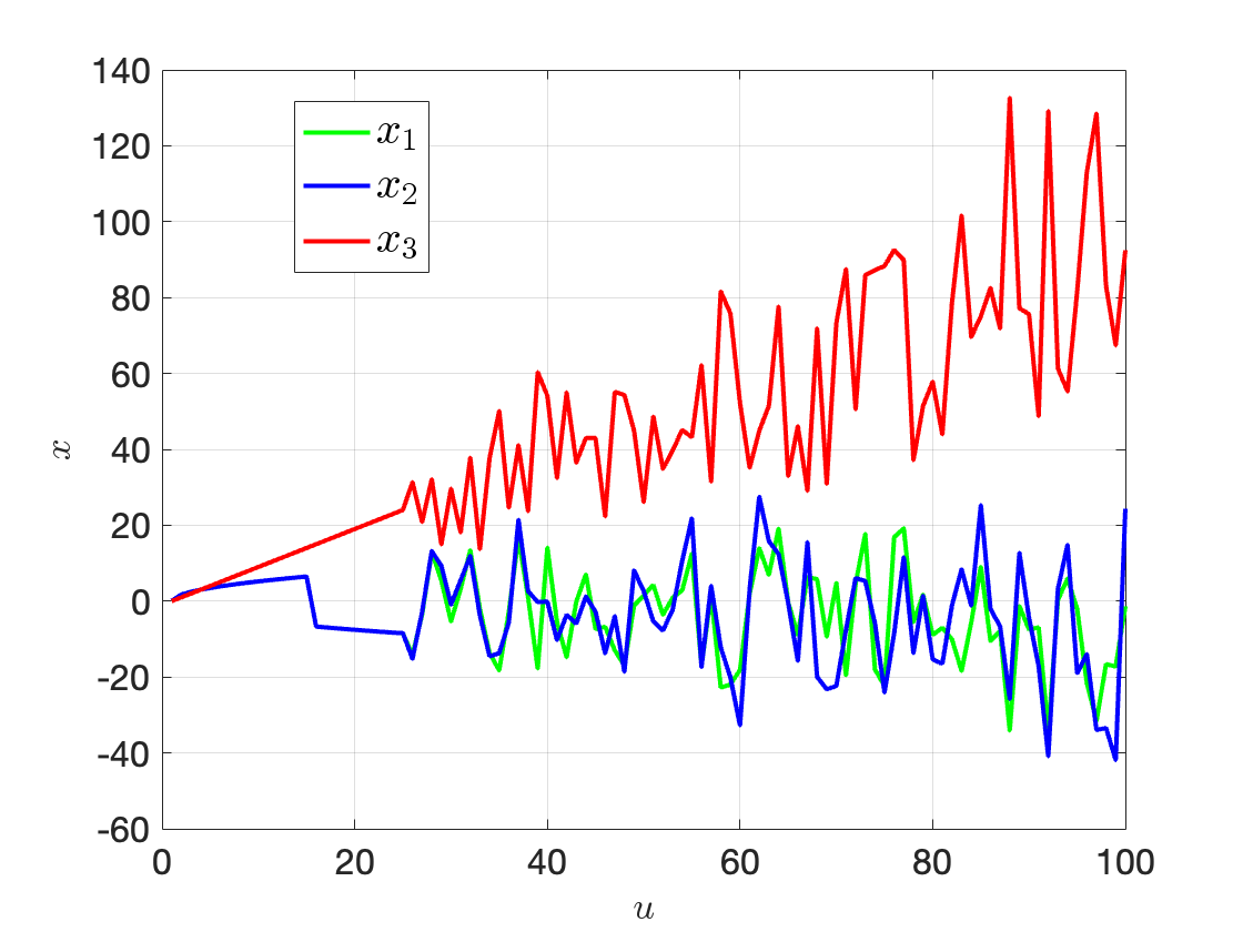
Figure 3.4: RK4 simulation.

3.2.2 Direct Multiple Shooting

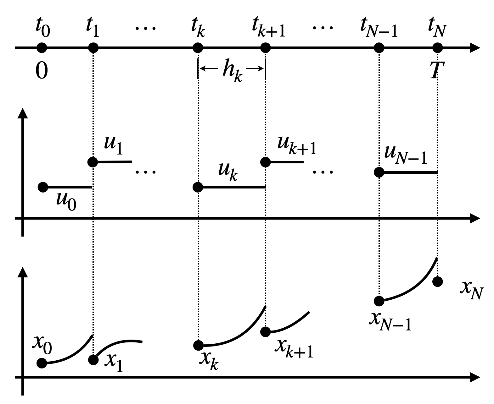
Figure 3.5: Direct multiple shooting.

Propagation of the nonlinearities through numerical integrators motivates using direct multiple shooting to transcribe the OCP problem into a nonlinear programming problem.

Instead of only optimizing the controls, direct multiple shooting optimizes both the controls and states. The decision variable in the NLP becomes \[ v = \begin{bmatrix} u_0 \\ u_1 \\ \vdots \\ u_{N-1} \\ x_1 \\ x_2 \\ \vdots \\ x_N \end{bmatrix} \in \mathbb{R}^{N(n+m)}. \] With the state variables also introduced in the optimization, we no longer need to recursively run the RK4 integrators. Instead, we just need to run it once and enforce \[ x_{k+1} = \text{RK4}(x_k, u_k), \] i.e., the current state and the next state satisfy the dynamics constraint. This is shown in Fig. 3.5.

In summary, the transcribed NLP for the OCP problem using direct multiple shooting becomes \[\begin{equation} \begin{split} \min_{v = (u_0,\dots,u_{N-1},x_1,\dots,x_N)} & \quad g_T(x_N) + \sum_{k=0}^{N-1} \frac{g(x_k,u_k) + g(x_{k+1},u_{k+1})}{2} h_k \\ \text{subject to} & \quad x_{k+1} = \text{RK4}(x_k, u_k), \quad k=0,\dots,N-1 \\ & \quad c^u_i (u_k) \geq 0, i=1,\dots,q_u, \quad k=0,\dots,N-1 \\ & \quad c^x_i(x_k) \geq 0, i=1,\dots,q_x, \quad k=1,\dots,N \\ & \quad \phi_i(x_k, u_k) \geq 0, i=1,\dots,q, \quad k=0,\dots,N. \end{split} \tag{3.15} \end{equation}\]

Direct multiple shooting avoids the recursion of numerical integrators such as RK4, but at the expense of introducing additional state variables in the NLP.

Let us try direct multiple shooting on the double integrator.

Example 3.6 (Direct Multiple Shooting for Minimum-Time Double Integrator) The double integrator has continuous-time dynamics (which you have already seen in Exercise 9.2): \[ \ddot{q} = u. \] In standard state-space form, the dynamics is linear \[ x = \begin{bmatrix} q \\ \dot{q} \end{bmatrix}, \quad \dot{x} = \begin{bmatrix} 0 & 1 \\ 0 & 0 \end{bmatrix} x + \begin{bmatrix} 0 \\ 1 \end{bmatrix} u. \]

Let us consider the minimum-time optimal control problem \[\begin{equation} \begin{split} \min_{u(t),t \in [0,T]} & \quad T \\ \text{subject to} & \quad \dot{x} = A x + Bu, \quad x(0) = x_0 \\ & \quad x(T) = 0 \\ & \quad u(t) \in [-1,1], \forall t \in [0,T]. \end{split} \end{equation}\] which seeks to get from the initial condition \(x_0\) to the origin as fast as possible.

You should know from our physics intuition that the optimal controller is bang-bang, i.e., the optimal control first accelerates (deaccelerates) using the maximum control and then reverses using the opposite maximum control.

Let’s see if we can obtain the optimal controller using direct multiple shooting.

In direct multiple shooting, we will optimize the control trajectory, the state trajectory, and the final time \(T\). We fix the number of intervals \(N\), and discretize \([0,T]\) evenly into \(N\) intervals, which leads to variables for the NLP as \[ v=(T,x_0,\dots,x_{N},u_0,\dots,u_N). \] We can easily enforce the control constraints: \[ u_k \in [-1,1],k=0,\dots,N, \] and the initial / terminal constraints \[ x_0 = x_0, \quad x_N = 0. \] The only nontrivial constraint is the dynamics constraint: \[ x_{k+1} = \text{RK4}(x_k,u_k),k=0,\dots,N-1. \]

The following script shows how to use the Matlab integrator ode45 to enforce the dynamics constraint.

function dx = double_integrator(t,states,v)
% return xdot at the selected times t and states, using information from v
% assume the controls in v define piece-wise constant control signal
T = v(1); % final time
N = (length(v) - 1) / 3; % number of knot points
u_grid = v(2+2*N:3*N+1); % N controls
t_grid = linspace(0,1,N)*T;
u_t = interp1(t_grid,u_grid,t,'previous'); % piece-wise constant
A = [0 1; 0 0];
B = [0; 1];
dx = A * states + B * u_t;
end

function [c,ceq] = double_integrator_nonlincon(v,initial_state)
% enforce x_k+1 = RK45(x_k, u_k); integration done using ode45
T = v(1); % final time
N = (length(v) - 1) / 3; % number of knot points
t_grid = linspace(0,1,N)*T;
x1 = v(2:N+1); % position 
x2 = v(2+N:2*N+1); % velocity
% u = v(2+2*N:3*N+1); % controls
% no inequality constraints
c = []; 
% equality constraints
ceq = [];
for i = 1:(N-1)
    ti = t_grid(i);
    tip1 = t_grid(i+1);
    xi = [x1(i);x2(i)];
    xip1 = [x1(i+1);x2(i+1)];
    % integrate system dynamics starting from xi in [ti,tip1]
    tt = ti:(tip1-ti)/20:tip1; % fine-grained time discretization
    [~,sol_int] = ode45(@(t,y) double_integrator(t,y,v),tt,xi);
    xip1_int = sol_int(end,:);
    % enforce them to be the same
    ceq = [ceq;
           xip1_int(1) - xip1(1);
           xip1_int(2) - xip1(2)];
end
% add initial state constraint
ceq = [ceq;
       x1(1) - initial_state(1);
       x2(1) - initial_state(2)];

% add terminal state constraint: land at origin
ceq = [ceq;
       x1(end);
       x2(end)]; 
end

I first define a function double_integrator that returns the continuous-time dynaimcs, and then in the nonlinear constraints function double_integrator_nonlincon I use ode45 to simulate the dynamics starting at \(x_k\) from \(t_k\) to \(t_{k+1}\):

[~,sol_int] = ode45(@(t,y) double_integrator(t,y,v),tt,xi);

The solution I got from ode45 should be equal to my decision state variable.

Running the complete code with \(x_0 = [-10;0]\) and \(N=51\), I obtain the control signal in Fig. 3.6, which is bang-bang.

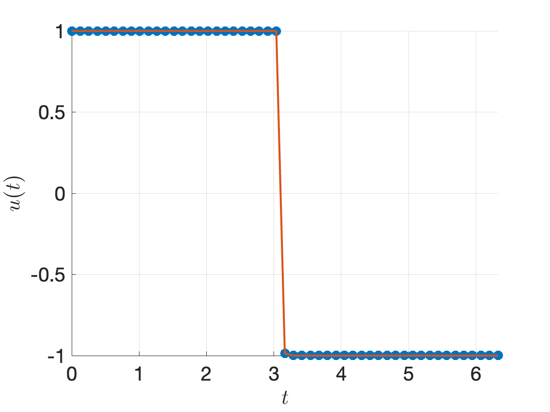
Figure 3.6: Optimal control signal by direct multiple shooting.

Using ode45 to integrate the double integrator dynamics from \(x_0\) with the controller in Fig. 3.6, we obtain the following state trajectory. Notice that the final state does not exactly land at the origin. This is expected due to our time discretization and imperfect dynamics integration using ode45. Make sure you play with the code, e.g., by changing the initial state \(x_0\) and see what happens.

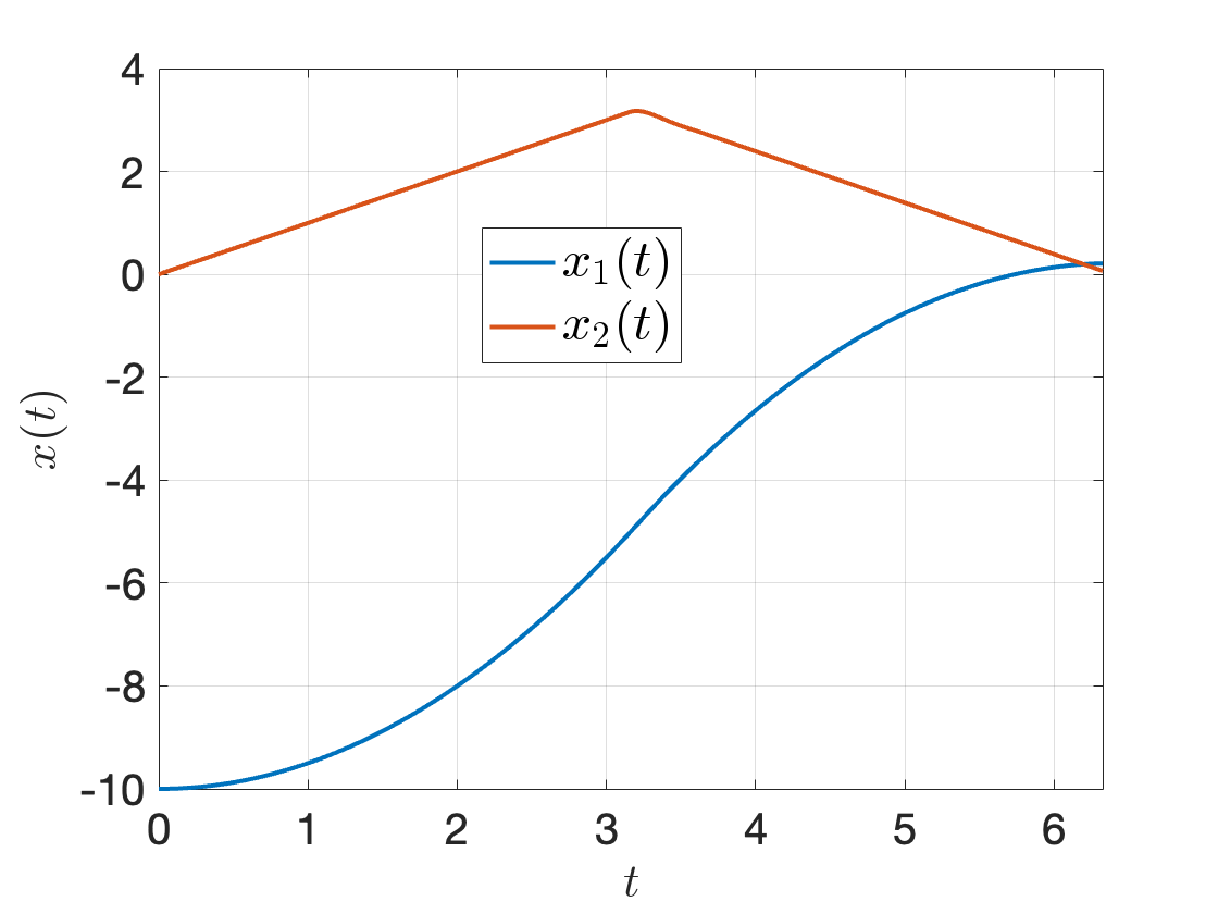
Figure 3.7: ODE45 integration with the optimal control signal found by direct multiple shooting.

3.2.3 Direct Collocation

In direct multiple shooting, we still need to rely on the numerical integrator RK4, which complicates the original nonlinear dynamics. In direct collocation, we will remove our dependency of RK4.

The key idea of direct collocation is to approximate the state trajectory \(x(t)\) and the control trajectory \(u(t)\) as piece-wise polynomial functions. In the following, we will describe the Hermite-Simpson collocation method.

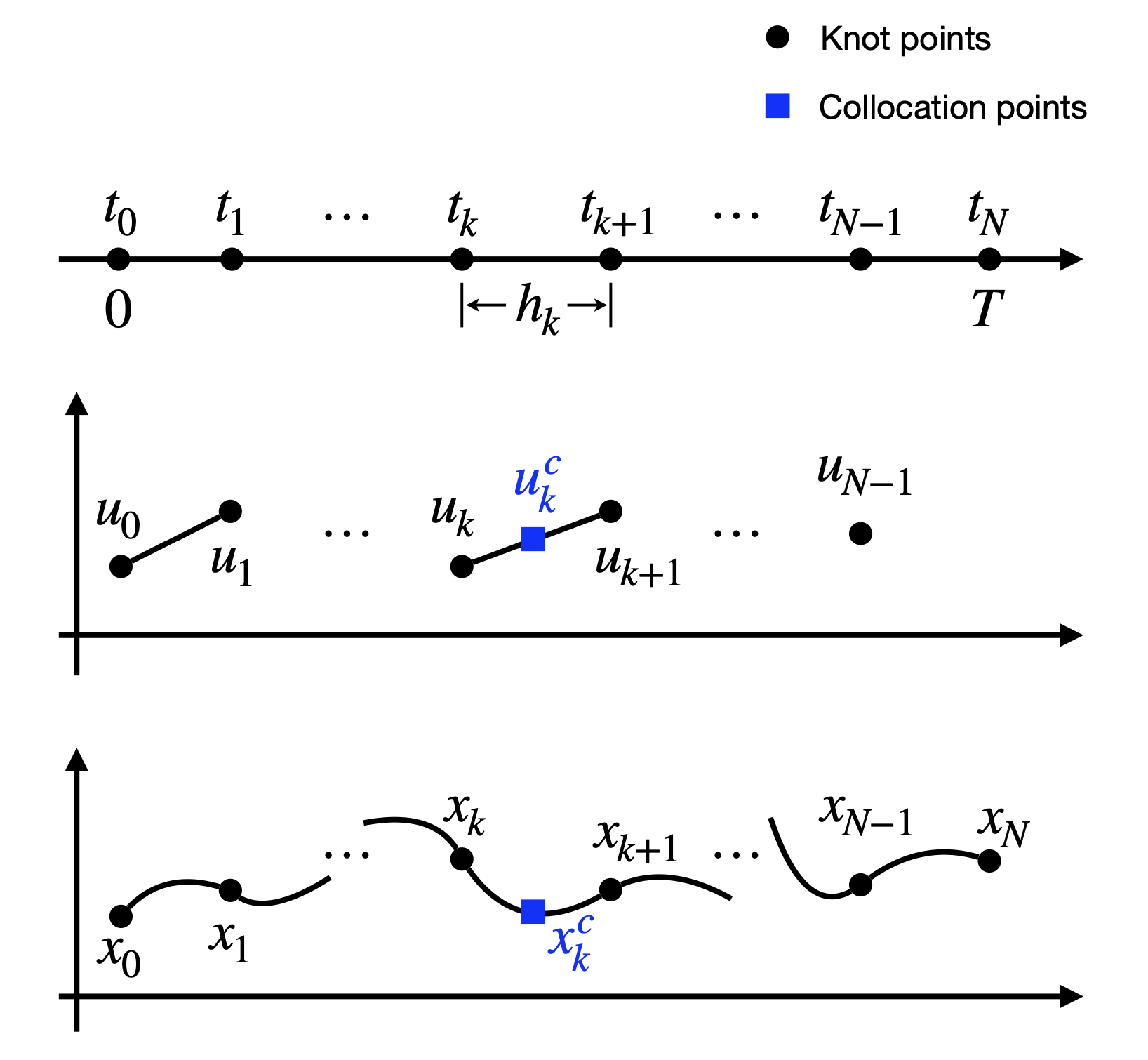
Figure 3.8: Direct collocation.

Time discretization. We first discretize the total time window \([0,T]\) into a set of \(N\) intervals: \[ 0 = t_0 \leq t_1 \leq \dots \leq t_k \leq t_{k+1} \leq \dots \leq t_N = T. \] We denote \[ h_k = t_{k+1} - t_k \] as the length of the \(k\)-th time interval. As we will see, the length of the time interval does not need to be fixed, and instead they can themselves be unknown variables to be optimized (in which case the final time \(T\) also becomes flexible).

Knot variables. At each of the timestamps \(t_0,\dots,t_N\), we assign knot variables, which are unknown state and control varaibles that need to be optimized. In particular, we have state knot variables \[ x_k = x(t_k), k=1,\dots,N, \] and control knot variables \[ u_k = u(t_k),k=0,\dots,N-1. \] As a result, the entire set of knot varaibles to be optimized is \[\begin{equation} v = \begin{bmatrix} u_0 \\ u_1 \\ \vdots \\ u_{N-1} \\ x_1 \\ x_2 \\ \vdots \\ x_{N} \end{bmatrix}. \tag{3.16} \end{equation}\] If the time-discretization is also optimized, then \(v\) includes the time intervals as well.

Transcribe dynamics. The most important step is to transcribe the nonlinear dynamics \(\dot{x}=f(x(t),u(t))\) as constraints on the knot varaibles. In direct collocation, the way this is done is to enforce the dynamics equation at the set of collocation points that are the mid-points between each consecutive pair of knot variables \((x_k, x_{k+1})\).

Specifically, in each subinterval \([t_k, t_{k+1}]\), we approximate the state trajectory as a cubic polynomial \[\begin{equation} x(t) = p_{k,0} + p_{k,1}(t-t_k) + p_{k,2}(t-t_k)^2 + p_{k,3}(t - t_k)^3, \quad t \in [t_k, t_{k+1}], \tag{3.17} \end{equation}\] where \(p_{k,0},p_{k,1},p_{k,2},p_{k,3} \in \mathbb{R}^n\) are the coefficients of the polynomial. You would think that we would need to optimize the coefficients as well, but actually we won’t need to, as will be shown soon. With this parameterization, we can obtain the time derivative of \(x(t)\) as \[\begin{equation} \dot{x}(t) = p_{k,1} + 2 p_{k,2}(t-t_k) + 3p_{k,3}(t - t_k)^2, \quad t \in [t_k, t_{k+1}]. \tag{3.18} \end{equation}\] Now the key step is to write the coefficients \(p_{k,0},p_{k,1},p_{k,2},p_{k,3}\) using our knot variables (3.16). To do so, we can invoke (3.17) and (3.18) to obtain \[ \begin{bmatrix} x_k \\ \dot{x}_k = f(x_k,u_k) \\ x_{k+1} \\ \dot{x}_{k+1} = f(x_{k+1}, u_{k+1}) \end{bmatrix} = \begin{bmatrix} I & 0 & 0 & 0 \\ 0 & I & 0 & 0 \\ I & h_k I & h_k^2 I & h_k^3 I \\ 0 & I & 2 h_k I & 3 h_k^2 I \end{bmatrix} \begin{bmatrix} p_{k,0}\\ p_{k,1}\\ p_{k,2}\\ p_{k,3} \end{bmatrix}. \] Solving the above equation, we get \[\begin{equation} \begin{bmatrix} p_{k,0}\\ p_{k,1}\\ p_{k,2}\\ p_{k,3} \end{bmatrix} = \begin{bmatrix} I & 0 & 0 & 0 \\ 0 & I & 0 & 0 \\ - \frac{3}{h_k^2} I & - \frac{2}{h_k} I & \frac{3}{h_k^2} I & -\frac{1}{h_k} I \\ \frac{2}{h_k^3} I & \frac{1}{h_k^2} I & -\frac{2}{h_k^3} I & \frac{1}{h_k^2} I \end{bmatrix} \begin{bmatrix} x_k \\ f(x_k,u_k) \\ x_{k+1} \\ f(x_{k+1}, u_{k+1}) \end{bmatrix}. \tag{3.19} \end{equation}\] Equation (3.19) implies, using the knot variables \(v\) in (3.16), we can query the value of \(x(t)\) and \(\dot{x}(t)\) at any time \(t \in [0,T]\). In particular, we will query the values of \(x(t)\) and \(\dot{x}(t)\) at the midpoints to obtain \[ x_k^c = x\left( t_k + \frac{h_k}{2} \right) = \frac{1}{2} (x_k + x_{k+1}) + \frac{h_k}{8} (f(x_k,u_k) - f(x_{k+1},u_{k+1})), \] and \[ \dot{x}_k^c = \dot{x} \left( t_k + \frac{h_k}{2} \right) = - \frac{3}{2h_k} (x_k - x_{k+1}) - \frac{1}{4} \left( f(x_k,u_k) + f(x_{k+1},u_{k+1}) \right). \] At the midpoint, we assume the control is \[ u_k^c = \frac{1}{2}(u_k + u_{k+1}). \] Therefore, we can enforce the dynamics constraint at the midpoint as \[\begin{equation} \dot{x}^c_k = f(x_k^c, u_k^c). \tag{3.20} \end{equation}\]

Transcribe other constraints. The other constraints in the continuous-time formulation (3.9) can be transcribed to the knot variables in a straightforward way: \[\begin{align} x_k \in \mathcal{X} \Rightarrow c_i^x(x_k)\geq 0, i=1,\dots,q_x, \quad k=1,\dots,N \\ u_k \in \mathcal{X} \Rightarrow c^u_i(u_k) \geq 0, i=1,\dots,q_u, \quad k=0,\dots,N-1\\ \phi_i(x_k, u_k) \geq 0, i=1,\dots,q, \quad k=0,\dots,N. \end{align}\]

Transcribe the objective. We can write the objective as \[ g_T(x_N) + \sum_{k=0}^{N-1} \frac{g(x_k,u_k) + g(x_{k+1},u_{k+1})}{2} h_k. \]

Summary. In summary, the final optimization problem becomes

\[\begin{equation} \begin{split} \min_{u_0,\dots,u_{N-1},x_1,\dots,x_N} & \quad g_T(x_N) + \sum_{k=0}^{N-1} \frac{g(x_k,u_k) + g(x_{k+1},u_{k+1})}{2} h_k \\ \text{subject to} & \quad \dot{x}_k^c = f(x_k^c,u_k^c), \quad k=0,\dots,N-1 \\ & \quad c_i^x(x_k) \geq 0,i=1,\dots,q_x, \quad k=1,\dots,N \\ & \quad c_i^u(u_k) \geq 0,i=1,\dots,q_u, \quad k=0,\dots,N-1 \\ & \quad \phi_i (x_k,u_k) \geq 0, i=1,\dots,q, \quad k=0,\dots,N. \end{split} \tag{3.21} \end{equation}\]

Let us apply direct collocation to the same double integrator Example 3.6.

Example 3.7 (Direct Collocation for Minimum-Time Double Integrator) Consider the same minimum-time optimal control problem in Example 3.6.

To apply direct collocation, we have our NLP variable \[ v = (T,x_0,\dots,x_N,u_0,\dots,u_N). \] Similarly we can enforce the control constraints and the initial / terminal constraints.

The following script shows how to enforce the collocation constraint.

function [c,ceq] = collocation(v,N,initial_state)
T = v(1);
h = T/(N-1);
x = reshape(v(2:2*N+1),2,N);
u = v(2*N+2:end);
c = [];
ceq = [];
for k=1:N-1
    uk = u(k);
    ukp1 = u(k+1);
    xk = x(:,k);
    xkp1 = x(:,k+1);
    fk = double_integrator(xk,uk);
    fkp1 = double_integrator(xkp1,ukp1);
    % collocation points
    xkc = 0.5*(xk+xkp1) + h/8 * (fk - fkp1);
    ukc = 0.5*(uk + ukp1);
    dxkc = -3/(2*h) * (xk-xkp1) - 0.25*(fk + fkp1);
    % collocation constraint
    ceq = [ceq;
           dxkc - double_integrator(xkc,ukc)];
end
ceq = [ceq;
       x(:,1) - initial_state; % initial condition
       x(:,end)]; % land at zero
end

As you can see, we do not need any numerical integrator such as ode45. The only thing we need is the continuous-time double integrator dynamics.

Running the complete code with \(x_0 = (-10,0)\) and \(N=51\), we get the control signal in Fig. 3.9 that is bang-bang.

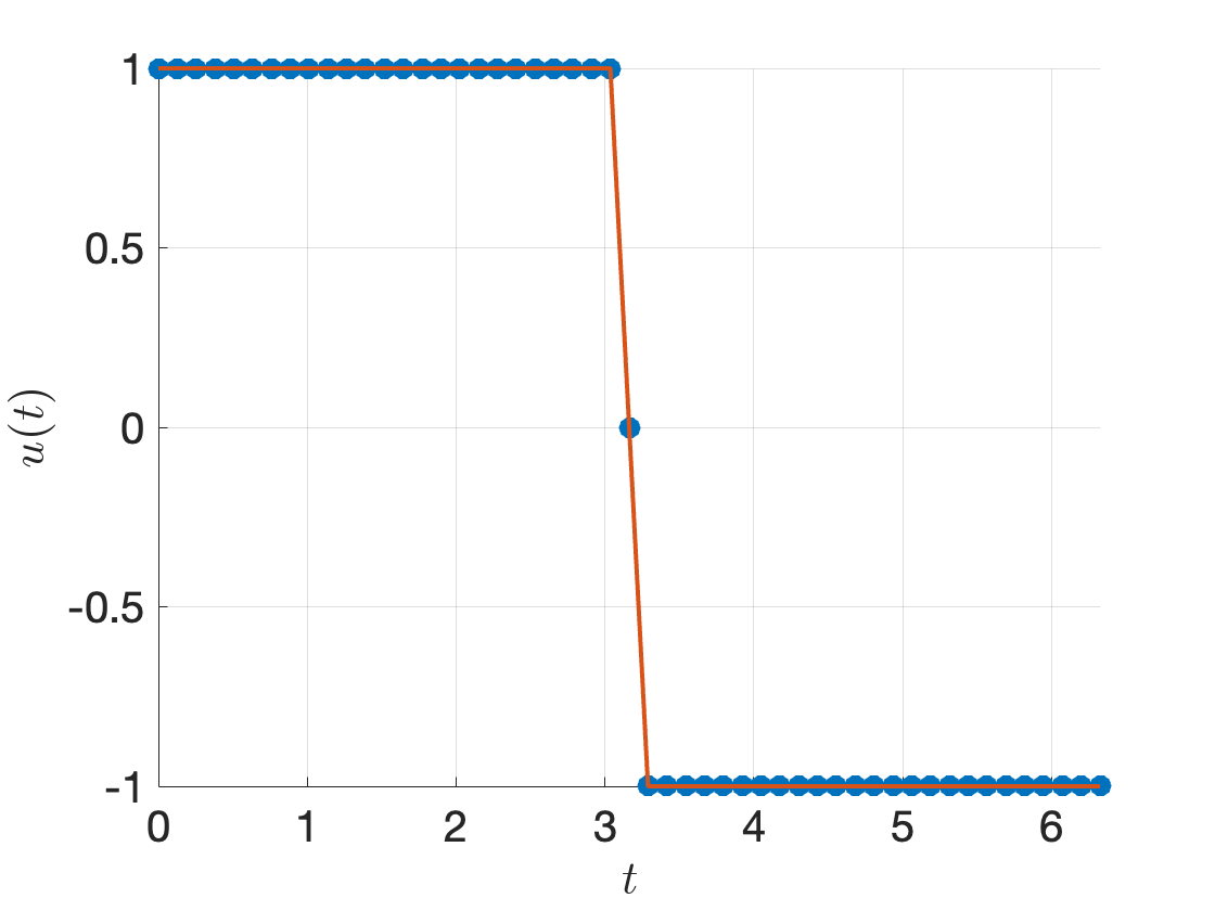
Figure 3.9: Optimal control signal by direct collocation.

Using ode45 to integrate the double integrator dynamics from \(x_0\) with the controller in Fig. 3.9, we obtain the following state trajectory. Comparing Fig. 3.10 with Fig. 3.7, we can observe that the terminal state of the trajectory obtained from direct collocation is more accurate than that obtained from direct multiple shooting.

Figure 3.10: ODE45 integration with the optimal control signal found by direct collocation.

Not only is direct collocation more accurate for this example, it is also faster. This is evident because in direct multiple shooting, evaluating the nonlinear constraints requires runing ode45, while in direct collocation, evaluating the nonlinear constraints simply requires calling the original continuous-time dynamics.

We can easily optimize with a larger \(N=101\) and get the following results.

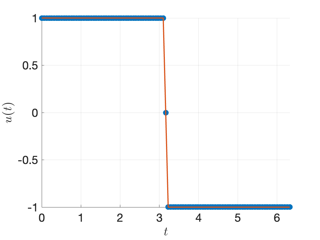
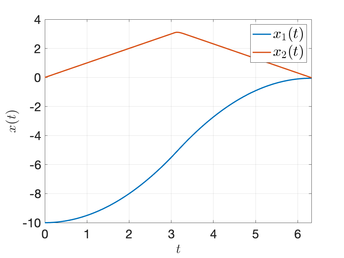
Figure 3.11: Direct collocation with N=101.

If you are interested in direct collocation, there is a nice tutorial with Matlab examples in (Kelly 2017).

3.2.4 Direct Orthogonal Collocation

3.2.5 Failure of Open-Loop Control

Trajectory optimization produces very satisfying trajectories when the nonlinear programming algorithms work as expected, as shown by the previous Examples 3.7 and 3.6 on the double integrator system.

However, does this imply that if we simply run the planned controls on a real system, i.e., doing open-loop control, the trajectory will behave as planned?

Unfortunately the answer is No, for two major reasons.

1. Trajectory optimization only produces an approximate solution to the optimal control problem (OCP) (3.9), regardless of what transcription method is used (such as multiple shooting and direct collocation). This means every \(u_k\) we obtained is an approximation to the true optimal controller \(u(t_k)\), and the approximation errors will accumulate as the dynamical system is evolving.

2. Even the OCP (3.9) is an imperfect approximation of the true control task. This is due to we assumed we have perfect knowledge of the system dynamics \[ \dot{x} = f(x(t),u(t)), \] which rarely holds in practice. For example, in the double integrator example, there is always friction between the mass and the ground. A more realistic assumption is that the system dynamics is \[ \dot{x} = f(x(t),u(t)) + w_t, \] where \(w_t\) is some unknown disturbance, or modeling error.

Let us observe the failure of open-loop control on our favorite pendulum example.

Example 3.8 (Failure of Open-Loop Control on A Simple Pendulum) Consider an “ideal” pendulum dynamics model \[ x = \begin{bmatrix} \theta \\ \dot{\theta} \end{bmatrix}, \quad \dot{x} = f(x,u) = \begin{bmatrix} \dot{\theta} \\ - \frac{1}{ml^2} (b \dot{\theta} + mgl \sin \theta) + \frac{1}{ml^2} u \end{bmatrix}, \] with \(m=1,l=1,g=9.8,b=0.1\). We enforce control saturation \[ u \in [-u_{\max}, u_{\max}] \] with \(u_{\max} = 4.9\).

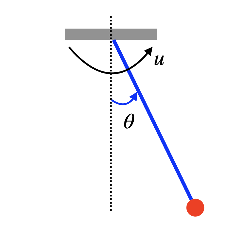
Figure 3.12: Simple pendulum.

Consider the optimal control problem with \(T=10\) \[\begin{equation} \begin{split} \min_{u(t), t \in [0,T]} & \quad \int_{t=0}^T (\cos \theta(t) + 1)^2 + \sin^2\theta(t) + \dot{\theta}^2(t) + u^2 dt \\ \text{subject to} & \quad \dot{x} = f(x(t),u(t)) \\ & \quad x(0) = [0,0]^T, \quad x(T) = [\pi,0]^T, \\ & \quad u(t) \in [-u_{\max},u_{\max}], \end{split} \tag{3.22} \end{equation}\] where we start from the initial state \([0,0]^T\), i.e., the bottomright position, and we want to swing up the pendulum to the final state \([\pi,0]^T\), i.e., the upright position. The cost function in (3.22) penalizes the deviation of the state trajectory from the target state (the target state has \(\cos \theta = -1\), \(\sin \theta = 0\) and \(\dot{\theta} = 0\)), together with the magnitude of control.

Trajectory optimization with direct collocation. We perform trajectory optimization for the OCP (3.22) with direct collocation. We choose \(N=101\) break points with \(h=0.1\) equal interval to discretize the time.

The result of trajectory optimization is shown in Fig. 3.13. We can see that the pendulum is perfectly swung up to \([\pi,0]^T\) and stabilized there.

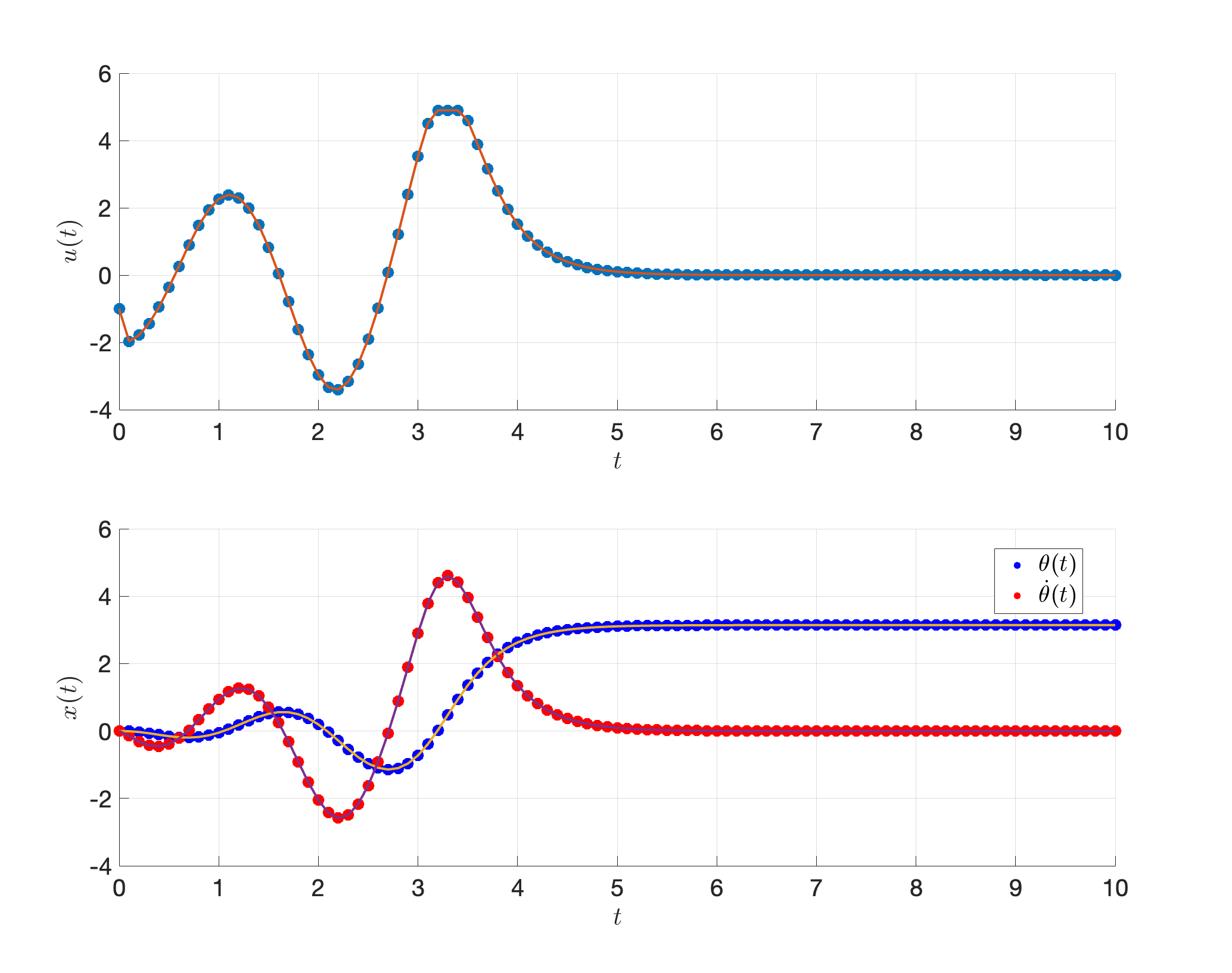
Figure 3.13: Pendulum swing-up with direct collocation

Deploy the optimized plan. We then deploy the optimized controls in Fig. 3.13 on the “ideal” pendulum. We deploy the control every \(0.1\) seconds with zero-order hold, and use Matlab ode89 to integrate the pendulum dynamics.

Fig. 3.14 shows the true trajectory of the pendulum. Unfortunately, the pendulum swing-up and stabilization is unsuccessful.

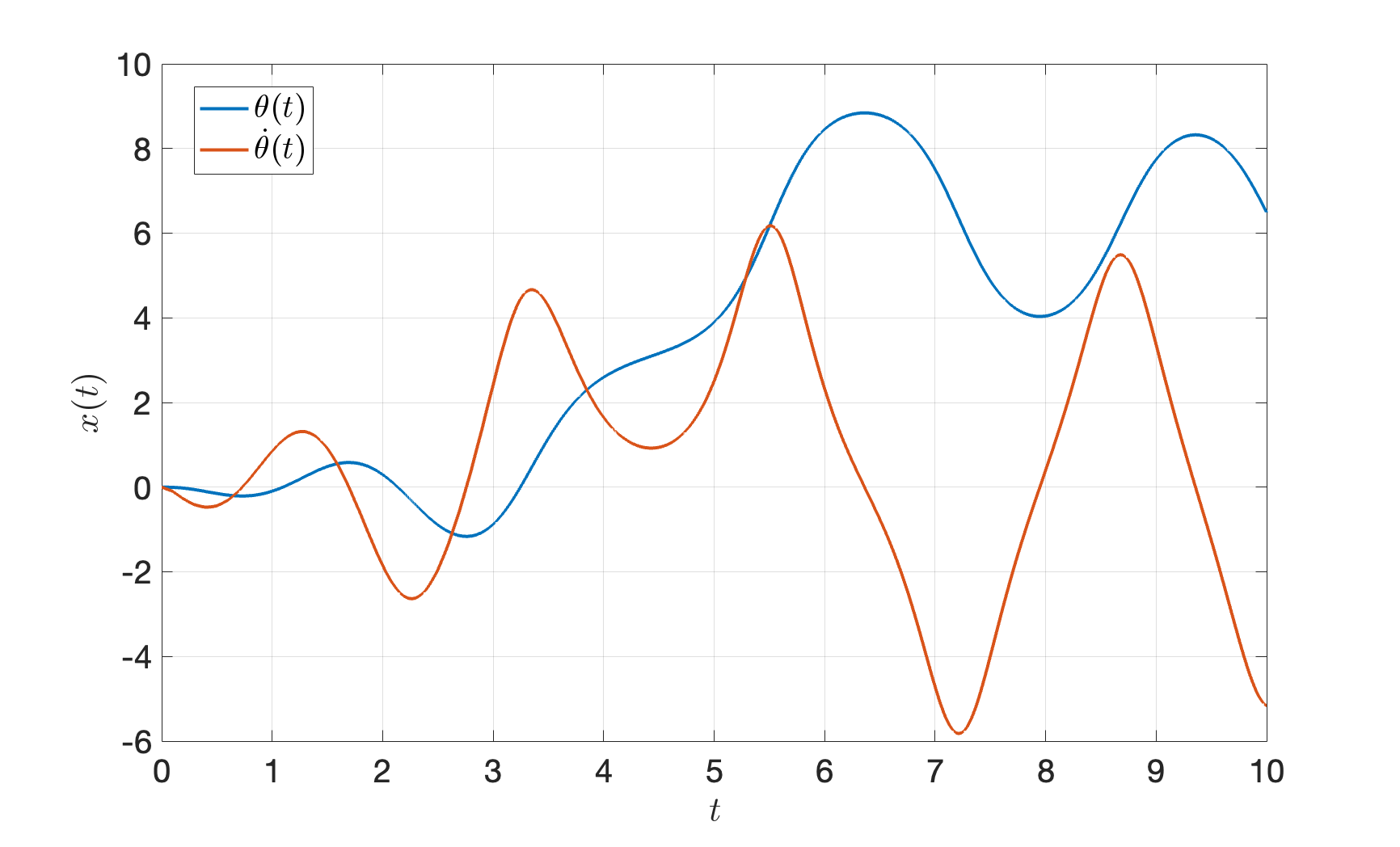
Figure 3.14: Deploy optimized controls

Adding noise. What if the true pendulum dynamics is \[ x = \begin{bmatrix} \theta \\ \dot{\theta} \end{bmatrix}, \quad \dot{x} = f(x,u) = \begin{bmatrix} \dot{\theta} \\ - \frac{1}{ml^2} (b \dot{\theta} + mgl \sin \theta) + \frac{1}{ml^2} u \end{bmatrix} + \begin{bmatrix} 0 \\ 1 \end{bmatrix}. \] That is, there is a constant unmodelled angular acceleration of \(1\), which maybe come from some unknown external force.

Fig. 3.15 shows the trajectory of the pendulum with the optimized controlls. We can clearly see the unmodelled dynamics makes the performance much worse.

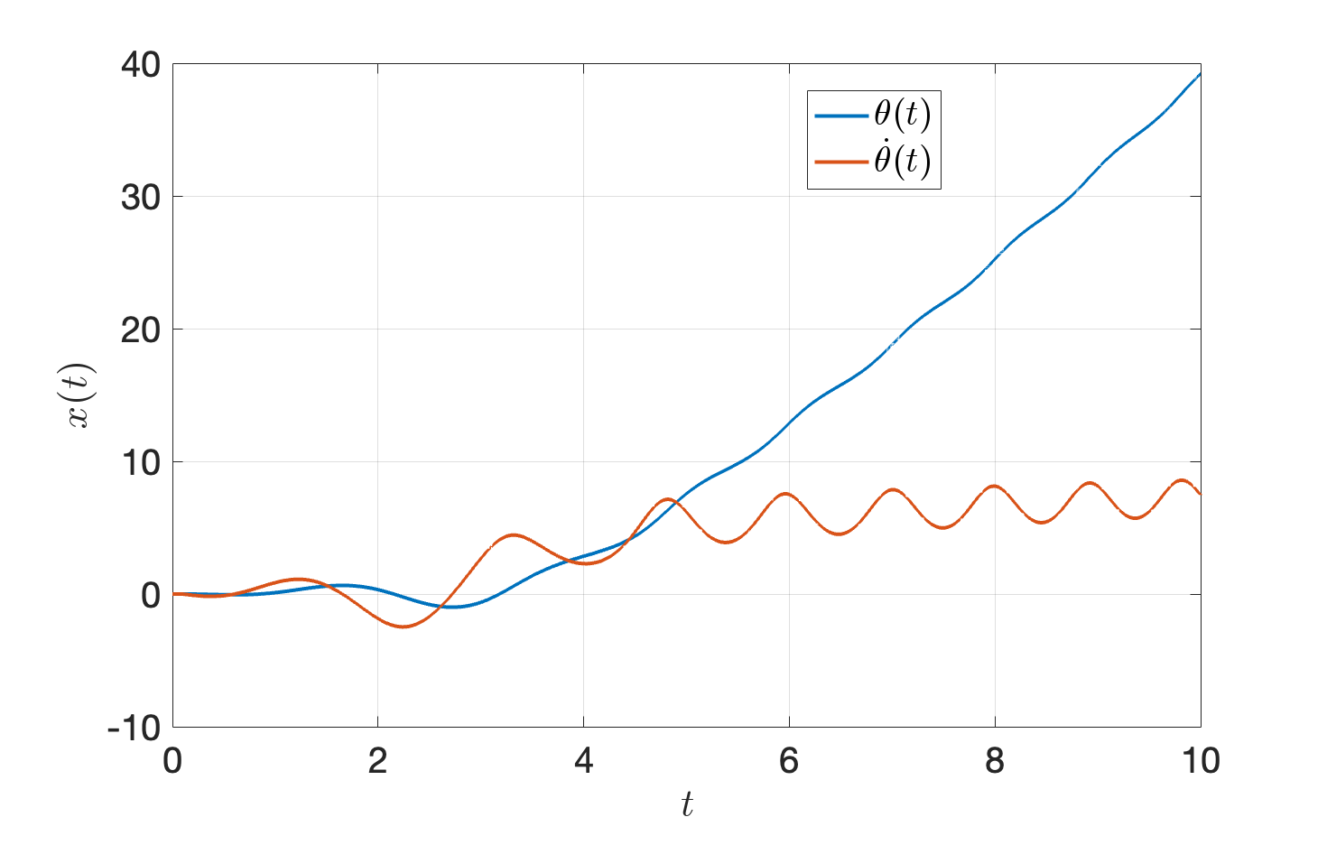
Figure 3.15: Deploy optimized controls on a system with disturbance

You can play with the code here.

The failure of open-loop control motivates feedback control.

3.2.6 LQR Trajectory Tracking

3.3 Model Predictive Control

The model predictive control framework leverages the idea of receding horizon control (RHC) to turn an open-loop controller into a closed-loop controller, i.e., a feedback controller.

For example, suppose we have an optimal control problem with horizon \(T\): \[\begin{equation} \begin{split} \min_{u(t), t \in [0,T]} & \quad g_T(x(T)) + \int_{t=0}^T g(x(t),u(t)) dt \\ \text{subject to} & \quad \dot{x} = f(x(t),u(t)), \quad x(0) = x_0 \\ & (x(t),u(t)) \in \mathcal{X} \times \mathcal{U}, \quad x(T) \in \mathcal{X}_T \end{split} \tag{3.23} \end{equation}\] where \(\dot{x} = f(x(t),u(t))\) is the best “ideal” model we have about our system.

The idea of RHC is as follows. At time \(t\), we obtain a measurement of the current state of the system, denoted as \(x_t\), and we solve the following OCP with horizon \(H < T\): \[\begin{equation} \begin{split} \min_{u(\tau), \tau \in [0,H]} & \quad g_t(x(H)) + \int_{\tau = 0}^H g(x(\tau),u(\tau)) d\tau \\ \text{subject to} & \quad \dot{x} = f(x(\tau),u(\tau)), \quad x(0) = x_t \\ & \quad (x(t),u(t)) \in \mathcal{X} \times \mathcal{U}, \quad x(H) \in \mathcal{X}_{t} \end{split} \tag{3.24} \end{equation}\] where notice that I used a different notation for the terminal cost \(g_t\) (as supposed to \(g_T\) in (3.23)), and the terminal constraint \(\mathcal{X}_t\) (as supposed to \(\mathcal{X}_T\) in (3.24)). Using a different terminal cost and terminal constraint is meant to make the problem (3.24) always feasible.

Suppose we solve the open-loop control problem (3.24) using trajectory optimization with \(N\) time intervals and obtained the following solution \[ u_{t,0},u_{t,1},\dots,u_{t,N}. \] Then RHS will only take the first control \(u_{t,0}\) and apply it to the system. Therefore, the closed-loop dynamics is effectively \[\begin{equation} \dot{x} = f(x(t),u_{t,0}), \tag{3.25} \end{equation}\] where \(u_{t,0}\) is the first control solution to the OCP (3.24).

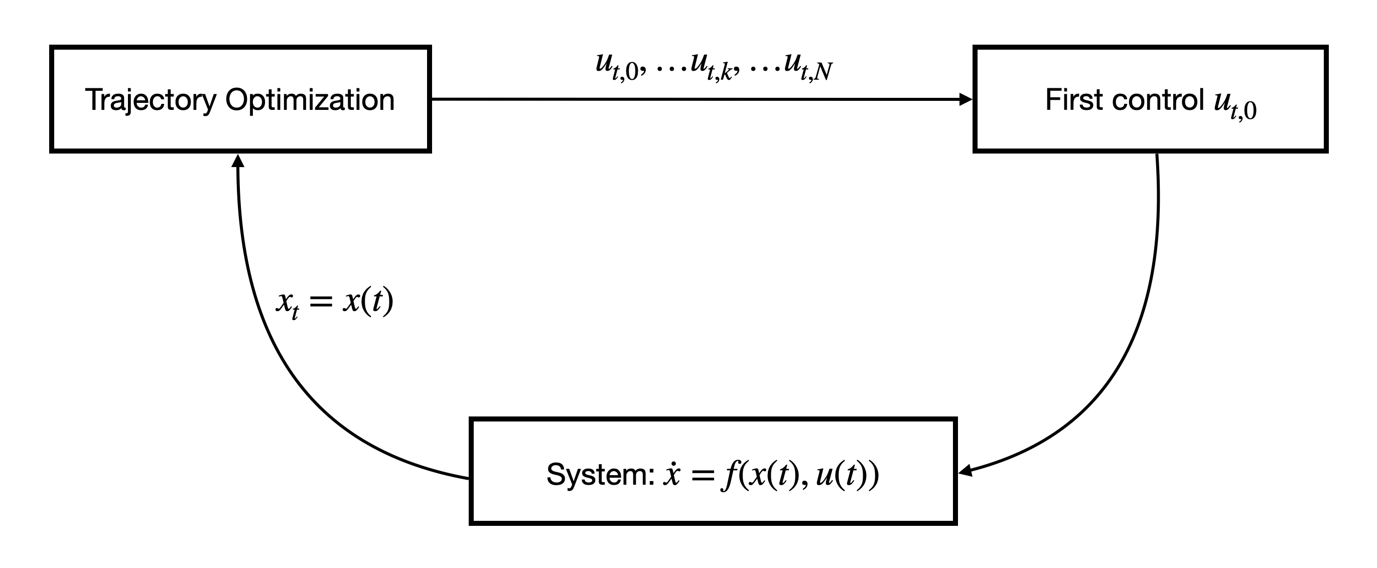
Figure 3.16: Receding horizon control

It is worth noting that RHS effectively introduces feedback control, because the controller \(u_{t,0}\) in (3.25) depends on \(x(t)\) via the open-loop optimal control problem (3.24).

Trajectory optimization and model predictive control are the workhorse for control of highly dynamic robots. For example, here is a talk by Scott Kuindersma on how trajectory optimization and model predictive control enable a diverse set of behaviors of Boston Dynamics’s humanoid robot.

3.3.1 Turn Trajectory Optimization into Feedback Control

Let us turn our trajectory optimization algorithm in Example 3.8 into a feedback controller through receding horizon control.

Example 3.9 (Pendulum Swingup with Model Predictive Control) Consider again the pendulum swingup task in Example 3.8.

This time, we will apply MPC to this task.

Again, we discretize the time windown \([0,T]\) into \(N-1 = 100\) equal intervals with \(h = 0.1\). At each timestep \(t_k = kh\), \(k=0,\dots,N-1\), we first measure the current state of the pendulum as \(x_k\), then solve the following OCP with planning horizon \(H=5\) \[\begin{equation} \begin{split} \min_{u(t), t \in [0,H]} & \quad \int_{t=0}^H (\cos \theta(t) + 1)^2 + \sin^2\theta(t) + \dot{\theta}^2(t) + u^2 dt \\ \text{subject to} & \quad \dot{x} = f(x(t),u(t)) \\ & \quad x(0) = x_k, \quad x(H) = [\pi,0]^T, \\ & \quad u(t) \in [-u_{\max},u_{\max}]. \end{split} \tag{3.26} \end{equation}\] We solve the OCP (3.26) using trajectory optimization with direct collocation (using \(M\) break points), which gives us a sequence of controls \[ u_{k,1},\dots,u_{k,M}, \] we deploy the first control \(u_{k,1}\) to the pendulum system.

MPC results. Fig. 3.17 shows the control and state trajectories when using MPC to swing up the pendulum. We can see that it works very well.

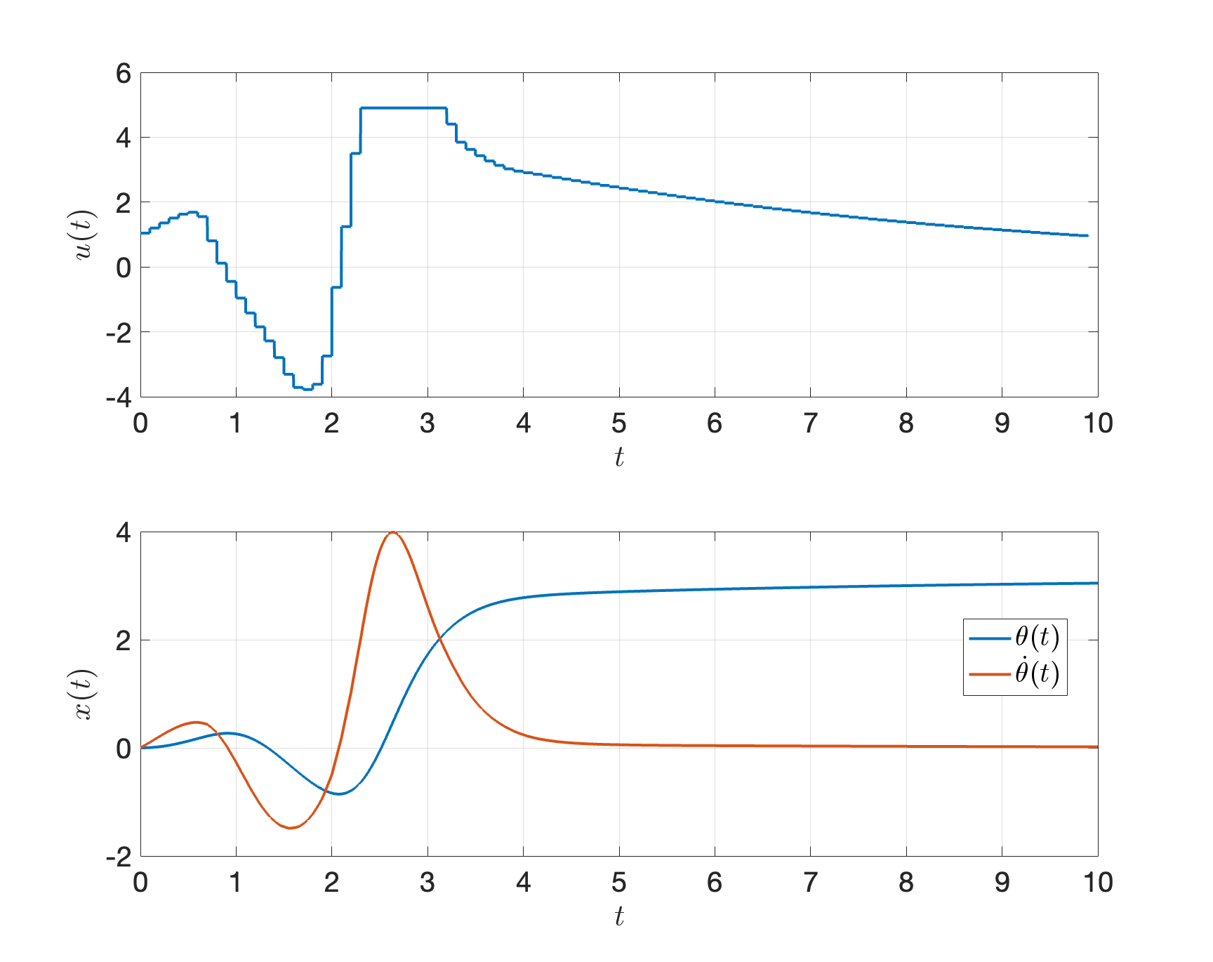
Figure 3.17: MPC for pendulum swing-up

Robustness to noise. MPC is naturally robust to modelling errors and noises. When the true system dynamics is \[ x = \begin{bmatrix} \theta \\ \dot{\theta} \end{bmatrix}, \quad \dot{x} = f(x,u) = \begin{bmatrix} \dot{\theta} \\ - \frac{1}{ml^2} (b \dot{\theta} + mgl \sin \theta) + \frac{1}{ml^2} u \end{bmatrix} + \begin{bmatrix} 0 \\ 1 \end{bmatrix}. \] The MPC controller still works very well, as shown in Fig. 3.18!

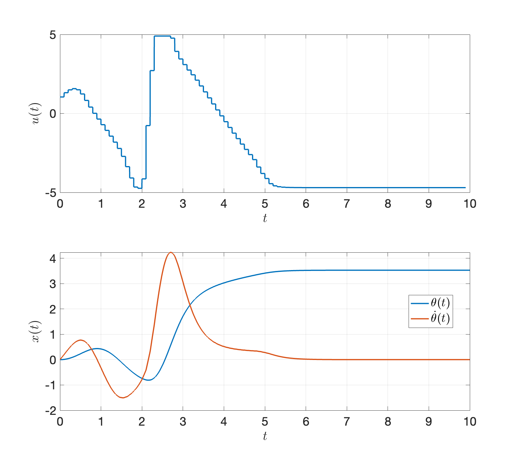
Figure 3.18: MPC for pendulum swing-up with noise

Feel free to play with the code here.

Software tools. Matlab implements a nice package for nonlinear MPC, you can refer to the documentation and examples. In Python, the do-mpc package is quite popular.

However, it is important to recognize that trajectory optimization for the nonconvex open-loop optimal control problen (3.24) (a) only guarantees a locally optimal solution and hence can be brittle, (b) can be time-consuming when the problem is high-dimensional.

In fact, MPC was originally developed in the context of chemical plant control (Borrelli, Bemporad, and Morari 2017), which has linear system dyanmics, as we will introduce soon. Before we introduce the MPC formulation and understand its theoretical properties, we need to take a detour and introduce various important notions of sets.

3.3.2 Controllability, Reachability, and Invariance

Consider the autonomous system \[\begin{equation} x_{t+1} = f_a(x_t) \tag{3.27} \end{equation}\] and the controlled system \[\begin{equation} x_{t+1} = f(x_t, u_t) \tag{3.28} \end{equation}\] for \(t \geq 0\). Both systems are subject to state and input constraints \[\begin{equation} x_t \in \mathcal{X}, \quad u_t \in \mathcal{U}, \forall t \geq 0, \tag{3.29} \end{equation}\] with \(\mathcal{X}\) and \(\mathcal{U}\) both being polyhedral sets (see Definition B.9) \[\begin{equation} \begin{split} x_t \in \mathcal{X} = \left\{ x \in \mathbb{R}^n \mid C x \leq c \right\}, \quad C \in \mathbb{R}^{l_x \times n}, c \in \mathbb{R}^{l_x}, \\ u_t \in \mathcal{U} = \left\{ u \in \mathbb{R}^m \mid D u \leq d \right\}, \quad D \in \mathbb{R}^{l_u \times m}, d \in \mathbb{R}^{l_u}. \end{split} \tag{3.30} \end{equation}\]

We are going to make a few definitions.

3.3.2.1 Controllable and Reachable Sets

Definition 3.1 (Precursor Set) For the autonomous system (3.27), we define the precursor set to a set \(\mathcal{S}\) as \[ \text{Pre}(\mathcal{S}) = \left\{ x \in \mathbb{R}^n \mid f_a(x) \in \mathcal{S} \right\}. \] In words, \(\text{Pre}(\mathcal{S})\) is the set of states which evolve into the target set \(\mathcal{S}\) in one time step.

For the controlled system (3.28), we define the precursor set to the set \(\mathcal{S}\) as \[ \text{Pre}(\mathcal{S}) = \left\{ x \in \mathbb{R}^n : \exists u \in \mathcal{U} \text{ s.t. } f(x,u) \in \mathcal{S} \right\}. \] In words, \(\text{Pre}(\mathcal{S})\) is the set of states that can be driven into the target set \(\mathcal{S}\) while satisfying control and state constraints.

A related concept is the successor set.

Definition 3.2 (Successor Set) For the autonomous system (3.27), we define the successor set to a set \(\mathcal{S}\) as \[ \text{Suc}(\mathcal{S}) = \left\{ x \in \mathbb{R}^n \mid \exists x' \in \mathcal{S} \text{ s.t. } x = f_a(x')\right\}. \] In words, the states in \(\mathcal{S}\) get mapped into the states in \(\text{Suc}(\mathcal{S})\) after one time step.

For the controlled system (3.28), we define the successor set to the set \(\mathcal{S}\) as \[ \text{Suc}(\mathcal{S}) = \left\{ x \in \mathbb{R}^n \mid \exists x' \in \mathcal{S}, \exists u' \in \mathcal{U} \text{ s.t. } x = f(x',u'). \right\} \] In words, the states in \(\mathcal{S}\) get mapped into the states in \(\text{Suc}(\mathcal{S})\) after one time step while satisfying the control constraints.

The \(N\)-step controllable set is defined by iterating \(\text{Pre}(\cdot)\) computations.

Definition 3.3 (N-Step Controllable Set) Let \(\mathcal{S} \subseteq \mathcal{X}\) be a target set. The \(N\)-step controllable set \(\mathcal{K}_{N}(\mathcal{S})\) of the system (3.27) or (3.28) subject to the constraints (3.29) is defined recursively as: \[ \mathcal{K}_0 (\mathcal{S}) = \mathcal{S}, \quad \mathcal{K}_{i}(\mathcal{S}) = \text{Pre}(\mathcal{K}_{i-1}(\mathcal{S})) \cap \mathcal{X}, i=1,\dots,N. \]

According to this definition, given any \(x_0 \in \mathcal{K}_N(\mathcal{S})\):

• For the autonomous system (3.27), its state will evolve into the target set \(\mathcal{S}\) in \(N\) steps while satisfying state constraints

• For the controlled system (3.28), there exists a sequence of admissible controls (i.e., satisfying control constraints) such that its state will evolve into the target set \(\mathcal{S}\) in \(N\) steps while satisfying state constraints.

Similarly, the \(N\)-step reachable set is defined by iterating \(\text{Suc}(\cdot)\) computations.

Definition 3.4 (N-Step Reachable Set) Let \(\mathcal{X}_0 \subseteq \mathcal{X}\) be an initial set. The \(N\)-step reachable set \(\mathcal{R}_N (\mathcal{X}_0)\) of the system (3.27) or (3.28) subject to the constraints (3.29) is defined recursively as: \[ \mathcal{R}_0(\mathcal{X}_0) = \mathcal{X}_0, \quad \mathcal{R}_{i}(\mathcal{X}_0) = \text{Suc}(\mathcal{R}_{i-1}(\mathcal{X}_0)) \cap \mathcal{X}, i=1,\dots,N. \]

According to this definition, given any \(x_0 \in \mathcal{X}_0\):

• For the autonomous system (3.27), its state will evolve into \(\mathcal{R}_N(\mathcal{X}_0)\) in \(N\) steps while satisfying state constraints

• For the controlled system (3.28), there exists a sequence of admissible controls (i.e., satisfying control constraints) such that its state will evolve into \(\mathcal{R}_N(\mathcal{X}_0)\) in \(N\) steps while satisfying state constraints.

In the literature, the controllable set is often referred to as the backwards reachable set.

3.3.2.2 Computation of Controllable and Reachable Sets

For a linear time-invariant system, when the state constraint set \(\mathcal{X}\), control constraint set \(\mathcal{U}\), the target set \(\mathcal{S}\), and the initial set \(\mathcal{X}_0\) are all polytopes, then the \(N\)-step controllable set \(\mathcal{K}_{N}(\mathcal{S})\) and the \(N\)-step reachable set \(\mathcal{R}_{N}(\mathcal{X}_0)\) are both polytopes and can be computed exactly and efficiently.

We will not describe the underlying algorithm for computing \(\mathcal{K}_{N}(\mathcal{S})\) and \(\mathcal{R}_{N}(\mathcal{X}_0)\) (these details can be found in (Borrelli, Bemporad, and Morari 2017) and they are not very difficult to understand, so I suggest you to read them), but we now show you how to use the Multi-Parametric Toolbox (MPT) to compute them.

Example 3.10 (Compute Controllable and Reachable Sets) Consider a linear system \[ x_{t+1} = \begin{bmatrix} 1.5 & 0 \\ 1 & -1.5 \end{bmatrix} x_t + \begin{bmatrix} 1 \\ 0 \end{bmatrix} u_t \] with state and control constraints \[ \mathcal{X} = [-10,10]^2, \quad \mathcal{U} = [-5,5]. \] Given \(\mathcal{S} = \mathcal{X}_0 = [-1,1]^2\), I want to compute \(\mathcal{K}_i(\mathcal{S})\) and \(\mathcal{R}_i(\mathcal{X}_0)\), for \(i=0,1,2,3,4\).

Dynamical system. We first define the linear time-invariant system as follows.

A = [1.5, 0; 1, -1.5]; B = [1; 0];
sys = LTISystem('A',A,'B',B);

We then define the state and control constraints.

calX = Polyhedron('A',...
    [1,0;0,1;-1,0;0,-1], ...
    'b',[10;10;10;10]);
calU = Polyhedron('A',[1;-1],'b',[5;5]);

Note that in the MPT toolbox, to define a polytope \(P = \{ x \in \mathbb{R}^n \mid A x \leq b \}\), we just need to call the Polyhedron function with inputs A and b.

Controllable sets. We have from Definition 3.3 the recursion \[ \mathcal{K}_0(\mathcal{S}) = \mathcal{S}, \quad \mathcal{K}_i(\mathcal{S}) = \text{Pre}(\mathcal{K}_{i-1}(\mathcal{S})) \cap \mathcal{X}. \] To implement the above set operation, we need two functions, one for the “\(\cap\)” intersection operation, and the other for the “\(\text{Pre}(\cdot)\)” precursor set operation. These two functions are both available through MPT.

• intersect(P,S) computes the intersection of two sets P and S, both defined as polytopes.

• system.reachableSet('X', X, 'U', U, 'N', 1, 'direction', 'backwards') computes the one-step backwards reachable set (which is just the precursor set) of the system with target set X and control constraints U.

Using these two functions, the following code snippet computes recursively the controllable sets for \(N\) steps.

% target set
S = Polyhedron('A',[1,0;0,1;-1,0;0,-1],'b',[1;1;1;1]);
K = [S];
N = 4;
for i = 1:N
    Si = sys.reachableSet('X',K(i),'U',calU,'N',1,'direction','backwards');
    K = [K; intersect(Si,calX)];
end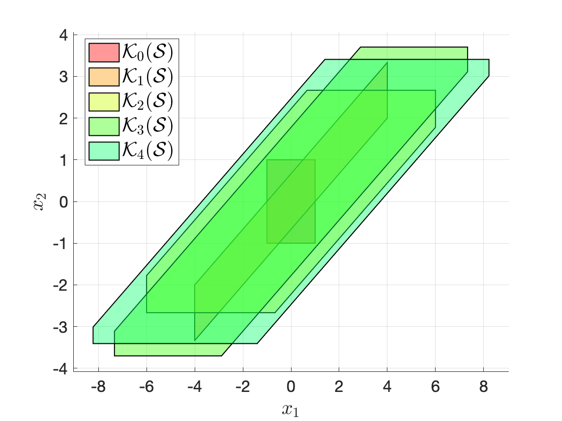

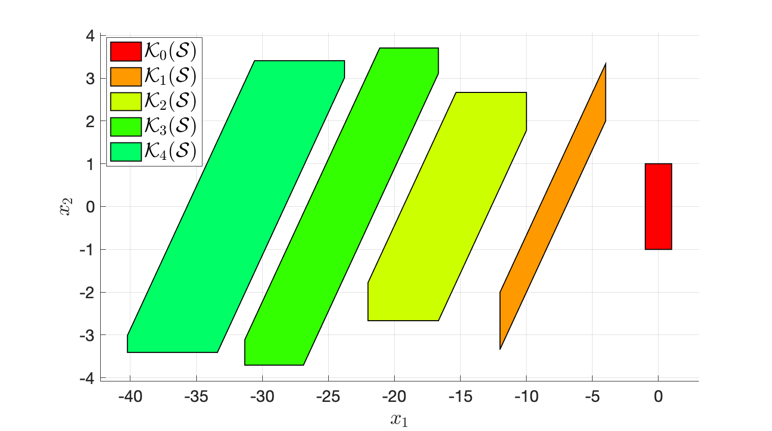
Fig. 3.19 plots the controllable sets computed by running the above code.

Figure 3.19: Computation of controllable sets using MPT. The bottom plot shifts the sets horizontally for better visualization.

Reachable sets. We have Definition 3.4 the recursion \[ \mathcal{R}_0(\mathcal{X}_0) = \mathcal{X}_0, \quad \mathcal{R}_i(\mathcal{X}_0) = \text{Suc}(\mathcal{R}_{i-1}(\mathcal{X}_0)) \cap \mathcal{X}. \] To implement the recursion above, we need “\(\cap\)” set intersection, which is available via intersect(P,S), and the “\(\text{Suc}(\cdot)\)” successor set operation, which is available as

• system.reachableSet('X', X, 'U', U, 'N', 1, 'direction', 'forward') computes the one-step forward reachable set (which is just the successor set) of the system with initial set X and control constraints U.

Therefore, we can compute the reachable sets recursively using the following code snippet

% initial set
X0 = Polyhedron('A',[1,0;0,1;-1,0;0,-1],'b',[1;1;1;1]);
R = [X0];
N = 4;
for i = 1:N
    Ri = sys.reachableSet('X',R(i),'U',calU,'N',1,'direction','forward');
    R = [R; intersect(Ri,calX)];
end

Fig. 3.20 plots the reachable sets computed by running the above code.

Feel free to play with the code here. Note that you need to install the MPT toolbox before running the code.

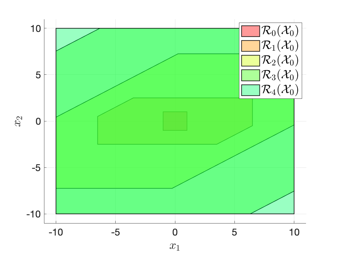
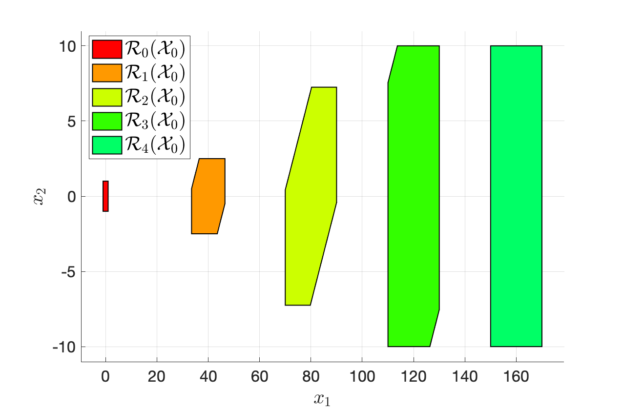
Figure 3.20: Computation of reachable sets using MPT. The bottom plot shifts the sets horizontally for better visualization.

3.3.2.3 Invariant Sets

Definition 3.5 (Positive Invariant Set) A set \(\mathcal{O} \subseteq \mathcal{X}\) is said to be a positive invariant set for the autonomous system (3.27) subject to the constraints in (3.29) if \[ x_0 \in \mathcal{O} \Longrightarrow x_t \in \mathcal{O}, \forall t \geq 0. \] That is, if the system starts in \(\mathcal{O}\), it stays in \(\mathcal{O}\) for all future timesteps.

The maximal positive invariant set is the largest positive invariant set.

Definition 3.6 (Maximal Positive Invariant Set) A set \(\mathcal{O}_{\infty} \subseteq \mathcal{X}\) is said to be the maximal positive invariant set for the autonomous system (3.27) subject to the constraints in (3.29) if (a) \(\mathcal{O}_{\infty}\) is positive invariant and (b) \(\mathcal{O}_{\infty}\) contains all the invariant sets contained in \(\mathcal{X}\).

Essentially, the (maximal) positive invariant set is the set of initial conditions under which the system does not blow up.

For the controlled system (3.28), we have the similar notion of a control invariant set.

Definition 3.7 (Control Invariant Set) A set \(\mathcal{C} \subseteq \mathcal{X}\) is said to be a control invariant set for the controlled system (3.28) subject to the constraints in (3.29) if \[ x_0 \in \mathcal{C} \Longrightarrow \exists u_t \in \mathcal{U} \text{ s.t. } f(x_t,u_t) \in \mathcal{C}, \forall t \geq 0 \] That is, if the system starts in \(\mathcal{C}\), it can be controlled to stay in \(\mathcal{C}\) for all future time steps.

The maximal control invariant set is the largest control invariant set.

Definition 3.8 (Maximal Control Invariant Set) A set \(\mathcal{C}_{\infty} \subseteq \mathcal{X}\) is said to be the maximal control invariant set for the controlled system (3.28) subject to the constraints in (3.29) if (a) \(\mathcal{C}_{\infty}\) is control invariant, and (b) \(\mathcal{C}_{\infty}\) contains all control invariant sets contained in \(\mathcal{X}\).

Essentially, the (maximal) control invariant set is the set of initial conditions under which the system can be controlled to not blow up.

We now state a necessary and sufficient condition for a set to be positive invariant and control invariant.

Theorem 3.1 (Geometric Condition for Invariance) For the autonomous system (3.27) subject to the constraint (3.29), a set \(\mathcal{O} \subseteq \mathcal{X}\) is positive invariant if and only if \[\begin{equation} \mathcal{O} \subseteq \text{Pre}(\mathcal{O}). \tag{3.31} \end{equation}\]

Similarly, for the controlled system (3.28) subject to the constraint (3.29), a set \(\mathcal{C}\) is control invariant if and only if \[\begin{equation} \mathcal{C} \subseteq \text{Pre}(\mathcal{C}). \tag{3.32} \end{equation}\]

Proof. We only prove (3.31) since (3.32) can be proved using similar arguments.

• “\(\Leftarrow\)”: we want to show \(\mathcal{O}\) is positive invariant if (3.31) holds. We prove this by contradiction. If \(\mathcal{O}\) is not positive invariant, the \(\exists \hat{x} \in \mathcal{O}\) such that \(f_a(\hat{x}) \not\in \mathcal{O}\). This implies we have found \(\hat{x} \in \mathcal{O}\) but \(\hat{x} \not\in \text{Pre}(\mathcal{O})\), contradicting (3.31).

• “\(\Rightarrow\)”: we want to show (3.31) holds if \(\mathcal{O}\) is positive invariant. We prove this by contradiction. Suppose (3.31) does not hold, then \(\exists \hat{x}\) such that \(\hat{x} \in \mathcal{O}\) but \(\hat{x} \not\in \text{Pre}(\mathcal{O})\). This implies we have found \(\hat{x} \in \mathcal{O}\) that does not remain in \(\mathcal{O}\) in the next step, contradicting \(\mathcal{O}\) being positive invariant.

This shows that (3.31) is a sufficient and necessary condition.

Theorem 3.1 immediately suggests an algoithm for computing (control) invariant sets, as we will describe in the next section.

3.3.2.4 Computation of Invariant Sets

Observe that the geometric conditions (3.31) and (3.32) are equivalent to the following conditions \[ \mathcal{O} = \text{Pre}(\mathcal{O}) \cap \mathcal{O}, \quad \mathcal{C} = \text{Pre}(\mathcal{C}) \cap \mathcal{C}. \]

Based on the equation above, we can design an algoithm that iteratively evaluates \(\text{Pre}(\mathcal{\Omega}) \cap \mathcal{\Omega}\) until it converges.

---

Algorithm: Computation of \(\mathcal{O}_{\infty}\)

---

Input: \(f_a\), \(\mathcal{X}\)

Output: \(\mathcal{O}_{\infty}\)

   \(\Omega_0 \leftarrow \mathcal{X}\), \(k=0\)

   Repeat

     \(\Omega_{k+1} \leftarrow \text{Pre}(\Omega_k) \cap \Omega_k\)

     \(k \leftarrow k+1\)

   Until \(\Omega_{k+1} = \Omega_k\).

   \(\mathcal{O}_{\infty} \leftarrow \Omega_k\)

---

The algorithm above generates a sequence of sets \(\{ \Omega_k \}\) satisfying \(\Omega_{k+1} \subseteq \Omega_k\) for any \(k\), and it terminates when \(\Omega_{k+1} = \Omega_k\). If it terminates, then \(\Omega_k\) is the maximal positive invariant set \(\mathcal{O}_{\infty}\). If \(\Omega_k = \emptyset\) for some intege \(k\) then \(\mathcal{O}_{\infty} = \emptyset\).

In general, the algoithm above may never terminate. If the algoithm does not terminate in a finite number of iterations, then it can be proven that (Kolmanovsky, Gilbert, et al. 1998) \[ \mathcal{O}_{\infty} = \lim_{k \rightarrow \infty} \Omega_k. \]

Conditions for finite time termination of the algoithm can be found in (Gilbert and Tan 1991). A simple sufficient condition requires the dynamics \(f_a\) to be linear and stable, and the constraint set \(\mathcal{X}\) to be bounded and contain the origin.

The same algoithm can be used to compute the maximal control invariant set \(\mathcal{C}_{\infty}\).

---

Algorithm: Computation of \(\mathcal{C}_{\infty}\)

---

Input: \(f\), \(\mathcal{X}\), \(\mathcal{U}\)

Output: \(\mathcal{C}_{\infty}\)

   \(\Omega_0 \leftarrow \mathcal{X}\), \(k=0\)

   Repeat

     \(\Omega_{k+1} \leftarrow \text{Pre}(\Omega_k) \cap \Omega_k\)

     \(k \leftarrow k+1\)

   Until \(\Omega_{k+1} = \Omega_k\).

   \(\mathcal{C}_{\infty} \leftarrow \Omega_k\)

---

Similarly, the above algoithm generates \(\{\Omega_k \}\) such that \(\Omega_{k+1} \subseteq \Omega_k\) for any \(k\). If the algoithm terminates, then \(\Omega_k = \mathcal{C}_{\infty}\).

In general, the algoithm may never terminate. If the algoithm does not terminate, then in general convergence is not guaranteed \[ \mathcal{C}_{\infty} \neq \lim_{k \rightarrow \infty} \Omega_k. \] The work in (Bertsekas 1972) reports examples of nonlinear systems for which the above equation can be observed. A sufficient condition for the convergence of \(\Omega_k\) to \(\mathcal{C}_{\infty}\) as \(k \rightarrow \infty\) requires the polyhedral sets \(\mathcal{X}\) and \(\mathcal{U}\) to be bounded and the system \(f(x,u)\) to be continuous (Bertsekas 1972).

Let us apply the algoithm to compute the maximal control invariant set for the linear system in Example 3.10.

Example 3.11 (Computation of the Maximal Control Invariant Set) Consider the linear system in Example 3.10 with same state constraint and control constraint.

The following code snippet shows how to apply the iterative algorithm introduced above to compute the maximal control invariant set.

Omega = [calX];
while true
    last_Omega = Omega(end);
    pre_omega = sys.reachableSet('X',last_Omega,'U',calU,'N',1,...
        'direction','backwards');
    new_Omega = intersect(pre_omega,last_Omega);
    Omega = [Omega;new_Omega];
    if new_Omega == last_Omega
        fprintf("Converged to maximal control invariant set.\n");
        break;
    end
end

The algoithm converges in 37 iterations and Fig. 3.21 plots the sequence of sets generated by the algorithm.

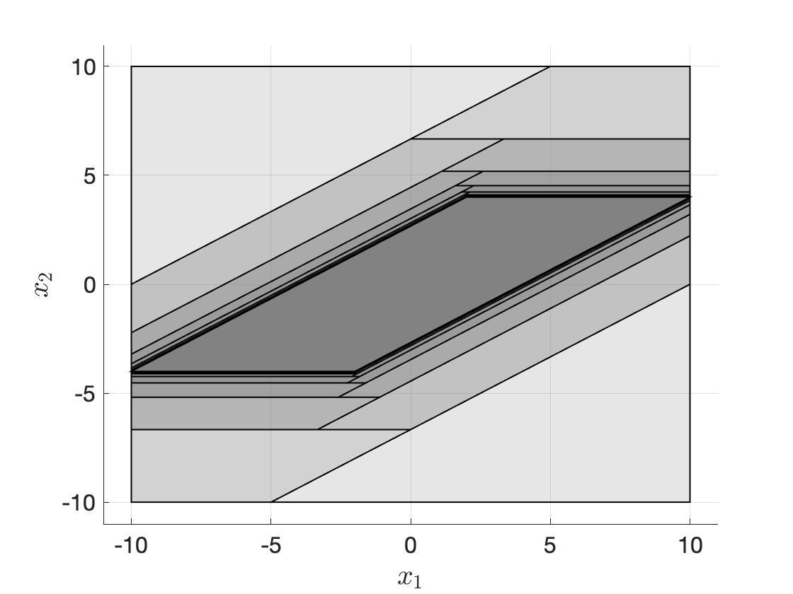
Figure 3.21: Maximal control invariant set.

The MPT toolbox actually implements this algoithm for us to use directly. If we use

C = sys.invariantSet('X', calX, 'U', calU);

we get the same result as before.

You can play with the code here.

3.3.3 Basic Formulation for Linear Systems

We are now ready to introduce the basic formulation of MPC for linear systems and study its theoretical properties.

Consider the problem of regulating the following discrete-time linear system to the origin \[\begin{equation} x_{t+1} = A x_t + B u_t, \tag{3.33} \end{equation}\] where the state \(x_t\) and control \(u_t\) are constrained to lie in polyhedral sets \(\mathcal{X}\) and \(\mathcal{U}\), respectively. We assume \(\mathcal{X}\) contains the origin \(0\).

We can formulate the following optimal control problem to regulate the system to the origin \[\begin{equation} \begin{split} J^\star(x_0) = \min_{u_t,t=0,\dots} & \quad \sum_{t=0}^{\infty} x_t^T Q x_t + u_t^T R u_t \\ \text{subject to} & \quad x_{t+1} = A x_t + B u_t, \\ & \quad (u_t,x_t) \in \mathcal{U} \times \mathcal{X}, \forall t = 0,\dots \end{split} \tag{3.34} \end{equation}\] with \(Q \succeq 0, R \succ 0\). Had we not included the constraints \((u_t,x_t) \in \mathcal{U} \times \mathcal{X}\), then problem (3.34) is exactly the infinite-horizon LQR problem in Section 2.1.1, for which we know the optimal controller is \(u_t = - K x_t\) with \(K\) computed in closed-form as (2.12).

However, in the presence of constraints, problem (3.34) does not admit a simple closed-form solution. In fact, problem (3.34) is commonly referred to as the contrained LQR (CLQR) problem and it is known that the optimal controller is piece-wise affine, see Theorem 11.4 in (Borrelli, Bemporad, and Morari 2017). We have asked you to numerically play with a toy example of CLQR in Exercise 9.2.

Receding horizon control. Leveraging the receding horizon control framework, we can approach problem (3.34) by online solving convex optimization problems.

At time \(t\), suppose we can measure the current state of the system \(x_t\), then we solve the following optimal control problem with a finite horizon \(N\) \[\begin{equation} \begin{split} J_t^\star(x_t) = \min_{u(0),\dots,u(N-1)} & \quad p(x(N)) + \sum_{k=0}^{N-1} q(x(k),u(k)) \\ \text{subject to} & \quad x(k+1) = A x(k) + B u(k), k =0, \dots, N-1, \quad x(0) = x_t \\ & \quad (x(k),u(k)) \in \mathcal{X} \times \mathcal{U}, k=0,\dots,N-1 \\ & \quad x(N) \in \mathcal{X}_f, \end{split} \tag{3.35} \end{equation}\] and \(p(x)\), \(q(x,u)\) convex functions. For example, a simple choice is \(p(x) = x^T P x\) and \(q = x^T Q x + u^T R u\) with \(P,Q\succeq 0\) and \(R \succ 0\). I hope you could pay attention to the notation in (3.35). I used \(x_t, u_t\) to denote the state and control for the original linear system (3.33) at time \(t\), as well as in the CLQR problem (3.34). However, in every subproblem (3.35) of RHS at time \(t\), I used \(x(k),u(k)\), with \(k\) as the time step, to denote the state and control in the finite-horizon optimal control problem starting at \(x_t\), with \(x_t = x(0)\) (\(k\) is the shifted time horizon in RHS that always starts at zero). In addition to the difference in notation between (3.35) and (3.34), problem (3.35) is also different in the following two ways:

1. Terminal cost \(p(x)\): in the objective of problem (3.35), there is an additional terminal cost \(p(x(N))\).

2. Terminal constraint set \(\mathcal{X}_f\): problem (3.35) has an additional constraint that the final state \(x(N)\) must belong to the set \(\mathcal{X}_f\). We assume \(\mathcal{X}_f\) is also polyheral (and convex).

Feasible sets. We denote as \(\mathcal{X}_0 \subseteq \mathcal{X}\) the set of initial states \(x_t\) such that the RHC subproblem (3.35) is feasible, i.e., \[\begin{equation} \hspace{-14mm} \begin{split} \mathcal{X}_0 = \{ x(0) \in \mathbb{R}^n \mid \exists (u(0),\dots,u(N-1)) \text{ such that } x(k) \in \mathcal{X},u(k) \in \mathcal{U},k=0,\dots,N-1, \\ x(N) \in \mathcal{X}_f \text{ with } x(k+1) = A x(k) + B u(k), k=0,\dots,N-1 \}. \end{split} \tag{3.36} \end{equation}\] Similarly, we denote as \(\mathcal{X}_i\) the set of states such that the RHC subproblem is feasible from step \(k=i\): \[\begin{equation} \hspace{-14mm} \begin{split} \mathcal{X}_i = \{ x(i) \in \mathbb{R}^n \mid \exists (u(i),\dots,u(N-1)) \text{ such that } x(k) \in \mathcal{X}, u(k) \in \mathcal{U}, k=i,\dots,N-1, \\ x(N) \in \mathcal{X}_f \text{ with } x(k+1) = A x(k) + B u(k), k=i,\dots,N-1 \}. \end{split} \tag{3.37} \end{equation}\] Clearly, by definition we have \[ \mathcal{X}_N = \mathcal{X}_f, \] and \[ \mathcal{X}_i = \{ x \in \mathcal{X} \mid \exists u \in \mathcal{U} \text{ such that } A x + Bu \in \mathcal{X}_{i+1} \},i=0,\dots,N-1, \] or written in a compact way as \[\begin{equation} \mathcal{X}_i = \text{Pre}(\mathcal{X}_{i+1}) \cap \mathcal{X}. \tag{3.38} \end{equation}\] Note that from equation (3.38) we have that, if we pick \(x_i \in \mathcal{X}_i\) and let \(U(x_i)\) be the set of feasible controls at \(x_i\), then pick any \((u(0),\dots,u(N-1)) \in U(x_i)\) and apply \(u(0)\) to the system to get \(x_{i+1} = A x_i + B u(0)\), we have \(x_{i+1} \in \mathcal{X}_{i+1}\).

Since the definitions (3.36) and (3.37) are rather abstract, let us visualize them using the double integrator example.

Example 3.12 (Double Integrator RHC Feasible Sets) Consider the discrete-time double integrator dynamics \[ x_{t+1} = \begin{bmatrix} 1 & 1 \\ 0 & 1 \end{bmatrix} x_t + \begin{bmatrix} 0 \\ 1 \end{bmatrix} u_t, \] subject to control constraint \[ u \in \mathcal{U} = [-0.5,0.5], \] and state constraint \[ x \in \mathcal{X} = [-5, 5] \times [-5, 5]. \] We use \(N=3\) and visualize the feasible sets (3.36) and (3.37) for two choices of \(\mathcal{X}_f\).

Choice 1. \(\mathcal{X}_f = \mathcal{X}\) is the full state space. We use the recursion (3.38) to compute the feasible sets \(\mathcal{X}_i\) for \(i=0,1,2,3\). Fig. 3.22 plots the feasible sets. Observe that in this case \(\mathcal{X}_0 \subset \mathcal{X}_1 \subset \mathcal{X}_2 \subset \mathcal{X}_3\). This creates a concern: suppose the RHC starts at \(x_0 \in \mathcal{X}_0\) that is feasible, in the next iteration we have \(x_1 \in \mathcal{X}_1\). However, since \(\mathcal{X}_1\) is larger than \(\mathcal{X}_0\), \(x_1\) is not guaranteed to be feasible.

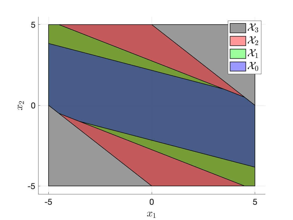
Figure 3.22: Feasible sets of the double integrator receding horizon controller without terminal constraint.

Choice 2. \(\mathcal{X}_f = \{(0,0)\}\) is the origin. Fig. 3.23 plots the feasible sets. Observe that in this case \(\mathcal{X}_3 \subset \mathcal{X}_2 \subset \mathcal{X}_1 \subset \mathcal{X}_0\). This is a nice case, because if RHC starts at \(x_0 \in \mathcal{X}_0\) that is feasible, in the next iteration we have \(x_1 \in \mathcal{X}_1 \subset \mathcal{X}_0\), which implies that \(x_1\) is guaranteed to remain feasible!

In fact, as we will soon show, in the first choice the RHC does suffer from infeasibility.

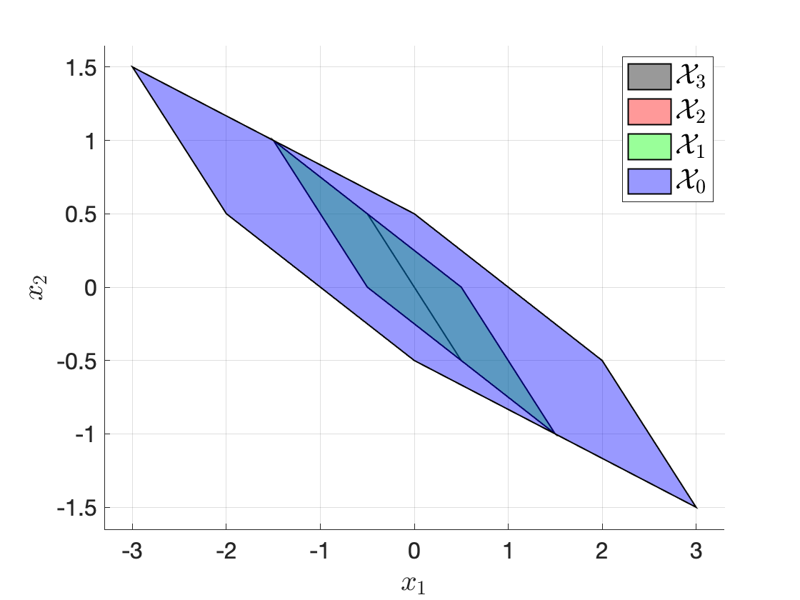
Figure 3.23: Feasible sets of the double integrator receding horizon controller with terminal constraint.

The code for this example can be found here.

Algorithm. Above all, problem (3.35) is a convex optimization problem that we know how to solve efficiently (you have solved such convex optimization problems in Exercise 9.2).

Let \(u^\star(0),\dots,u^\star(N-1)\) be the optimal solution of problem (3.35) when it is feasible, the RHS framework will only apply the first control \(u^\star(0)\) to the system, and hence the closed-loop system is \[\begin{equation} x_{t+1} = A x_t + u^\star_{x_t}(0) = f_{\mathrm{cl}}(x_t), \tag{3.39} \end{equation}\] where I have used \(u^\star_{x_t}(0)\) to make it explicit that the control is the first optimal control of solving (3.35) with an initial state \(x_t\). The following algorithm summarizes the receding horizon control algorithm.

---

Algorithm: Online Receding Horizon Control

---

Input: State \(x_t\) at time \(t\)

Output: Control \(u^\star_{x_t}(0)\)

1. Solve problem (3.35) to get the optimal controls \(u^\star(0), \dots, u^\star(N-1)\)
2. if the problem is infeasible, then stop
3. else return \(u^\star_{x_t}(0) = u^\star(0)\)

---

RHC main questions. Two main questions arise regarding the RHC controller.

1. Persistent feasibility. If the RHC algorithm starts at a state \(x_0\) for which the convex optimization (3.35) is feasible, i.e., \(x_0 \in \mathcal{X}_0\), will the convex optimization (3.35) remain feasible for all future time steps?

2. Stability. Assuming the convex optimization is always feasible. Will the closed-loop system (3.39) (induced by the RHC controller) converge to the desired origin \(x=0\)?

Let us use a couple of examples to illustrate that, in general, the answers to the above two questions are both NO.

Example 3.13 (Receding Horizon Control for Double Integrator) Consider the discrete-time double integrator dynamics \[ x_{t+1} = \begin{bmatrix} 1 & 1 \\ 0 & 1 \end{bmatrix} x_t + \begin{bmatrix} 0 \\ 1 \end{bmatrix} u_t, \] subject to control constraint \[ u \in \mathcal{U} = [-0.5,0.5], \] and state constraint \[ x \in \mathcal{X} = [-5, 5] \times [-5, 5]. \] In the RHS subproblem (3.35), we use \(N = 3\), \(p(x) = x^T P x\), \(q(x,u) = x^T Q x + u^T R u\) with \(P = Q = I\), \(R=10\), and \(\mathcal{X}_f = \mathbb{R}^2\) (i.e., there is not terminal constraint). The subproblem is implemented using CVX in Matlab.

Fig. 3.24 shows the state trajectory of executing RHC starting at \(x_0 = [-4.5;2]\) and \(x_0 = [-4.5;3]\), respectively.

We can see that when the initial state is \(x_0 = [-4.5;2]\), the trajectory successfully converges to the origin (the blue line). However, when the initial state is \(x_0 = [-4.5;3]\), RHC fails in the third iteration because the subproblem becomes infeasible (the red line).

You can find code for this example here.

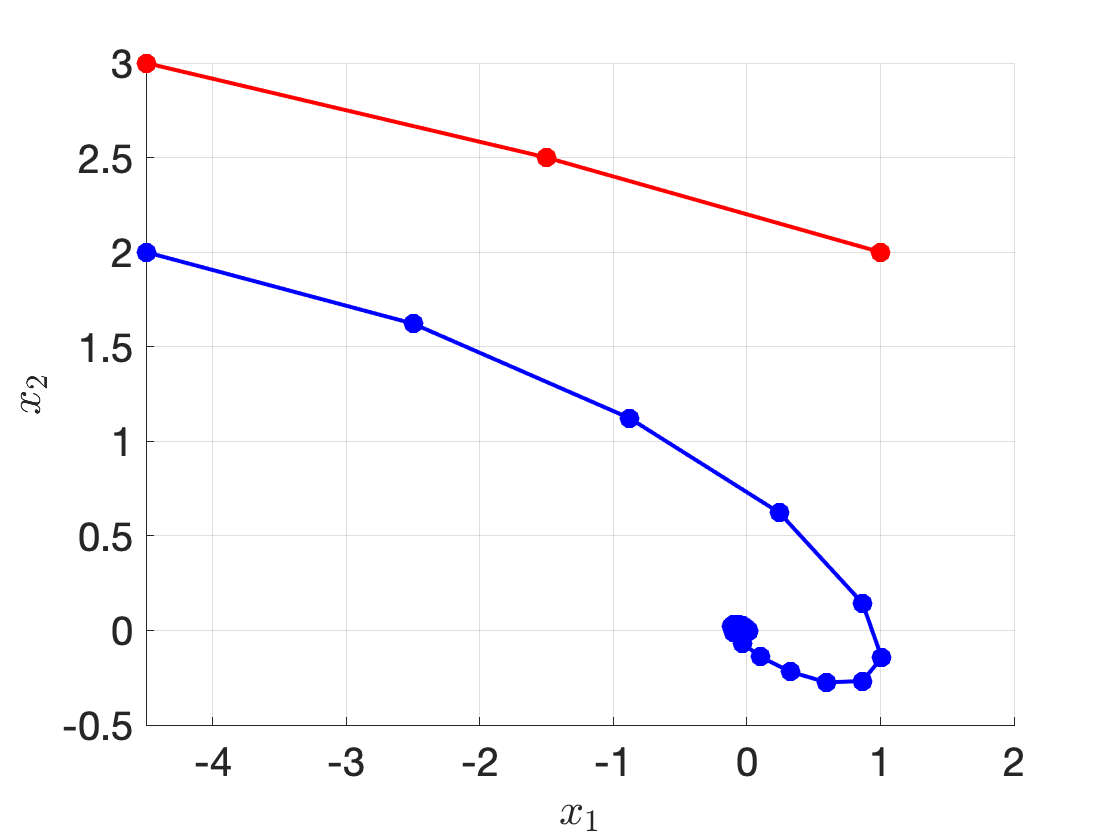
Figure 3.24: Receding horizon control for the double integrator with two initial states.

We now show another example, adapted from (Borrelli, Bemporad, and Morari 2017) where the design of \(N\), \(p(x)\) and \(q(x,u)\) affects the closed-loop performance.

Example 3.14 (RHC Performance Affected by Parameters) Consider the system \[ x_{t+1} = \begin{bmatrix} 2 & 1 \\ 0 & 0.5 \end{bmatrix} x_t + \begin{bmatrix} 1 \\ 0 \end{bmatrix} u_t, \] with control constraint \[ u \in \mathcal{U} = [-1,1], \] and state constraint \[ x \in \mathcal{X} = [-10,10] \times [-10,10]. \]

In the RHC problem (3.35), we choose \(p(x) = x^T P x\), \(q(x,u) = x^T Q x + u^T R u\). We fix \(P=0\), \(Q = I\), and \(\mathcal{X}_f = \mathbb{R}^2\), but vary \(N\) and \(R\):

• Setting 1: \(N=2\), \(R = 10\);

• Setting 2: \(N=3\), \(R = 2\);

• Setting 3: \(N=4\), \(R=1\).

Fig. 3.25 shows the closed-loop trajectories of three different settings. As we can see, the closed-loop performance depends on the parameters in a very complicated manner.

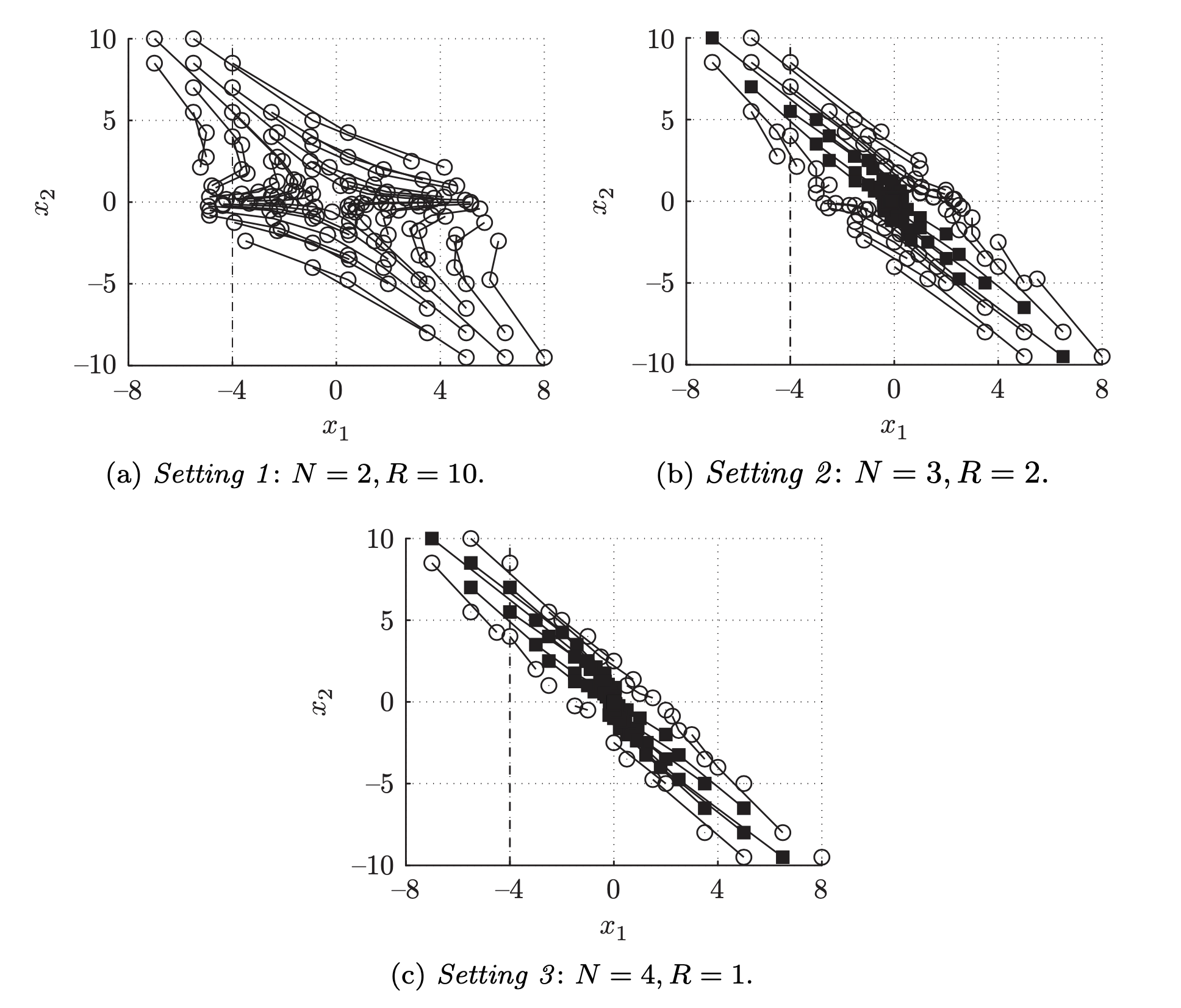
Figure 3.25: Closed-loop trajectories for different settings of horizon N and weight R. Boxes (circles) are initial points leading to feasible (infeasible) closed-loop trajectories.

3.3.4 Persistent Feasibility

Under what conditions can we guarantee the RHC subproblem (3.35) is always feasible?

Intuitively, we will show that, by designing the terminal constraint set \(\mathcal{X}_f\), we can guarantee the configuration of the feasible sets will look like choice 2 in Example 3.12.

There are various sets here of interest for answering this question.

• \(\mathcal{C}_{\infty}\): The maximal control invariant set \(\mathcal{C}_{\infty}\) is only affected by the system dynamics (3.33) and the constraint sets \(\mathcal{X} \times \mathcal{U}\). It is the largest set over which we can expect any controller to work, because otherwise the system trajectory will blow up.

• \(\mathcal{X}_0\): The set of states at which the RHC subproblem (3.35) is feasible. The set \(\mathcal{X}_0\) depends on the system dynamics, the constraint sets \(\mathcal{X} \times \mathcal{U}\), as well as the RHC horizon \(N\) and the terminal constraint set \(\mathcal{X}_f\). It is worth noting that it does not depend on the objective function in (3.35) (i.e., \(P,Q,R\)).

• \(\mathcal{O}_{\infty}\): The maximal positive invariant set for the closed-loop system (3.39) induced by the RHC control law. This depends on the RHC controller and hence it depends on the system dynamics, the constraint set \(\mathcal{X} \times \mathcal{U}\), \(N\), \(\mathcal{X}_f\) and the objective function of (3.35) \(P,Q,R\).

A few relationships between these sets are easy to observe.

• \(\mathcal{O}_{\infty} \subseteq \mathcal{X}_0\). Any state \(x \in \mathcal{O}_{\infty}\) needs to stay in \(\mathcal{O}_{\infty}\) for all future time steps. Thus, the subproblem (3.35) must be feasible for any \(x \in \mathcal{O}_{\infty}\), otherwise the closed-loop system (3.39) is not even well defined.

• \(\mathcal{O}_{\infty} \subseteq \mathcal{C}_{\infty}\). The set \(\mathcal{O}_{\infty}\) is control invariant because there exists a controller (specifically, the RHC controller) that makes it positive invariant. Therefore, \(\mathcal{O}_{\infty}\) must belong to the maximal control invariant set \(\mathcal{C}_{\infty}\).

We can now state necessary and sufficient conditions guaranteeing persistent feasibility.

Lemma 3.1 (Sufficient and Necessary Condition for Persistent Feasibility) The RHC subproblem (3.35) is persistently feasible if and only if \(\mathcal{X}_0 = \mathcal{O}_{\infty}\).

Proof. We have already argued that \(\mathcal{O}_{\infty} \subseteq \mathcal{X}_0\). It remains to show \(\mathcal{X}_0 \subseteq \mathcal{O}_{\infty}\). By definition, \(\mathcal{X}_0\) is persistently feasible implies that \[ x \in \mathcal{X}_0 \Longrightarrow f_{\mathrm{cl}}^t(x) \in \mathcal{X}_0, \forall t \] where \(f_{\mathrm{cl}}^t\) means applying the closed-loop dynamics \(f_{\mathrm{cl}}\) in (3.39) \(t\) times. This shows that \(\mathcal{X}_0\) is a positive invariant set for the closed-loop system, and hence \(\mathcal{X}_0 \subseteq \mathcal{O}_{\infty}\).

We argued that \(\mathcal{X}_0\) does not depend on the RHC parameters \(P,Q,R\) but \(\mathcal{O}_{\infty}\) does. Therefore, in general only some \(P,Q,R\) are allowed for persistent feasibility to hold. Due to the complicated relationship between \(P,Q,R\) and \(\mathcal{O}_{\infty}\), it is generally difficult to design \(P,Q,R\) such that RHC has persistent feasibility.

We now state a sufficient condition for persistent feasibility to hold.

Lemma 3.2 (Sufficient Condition for Persistent Feasibility) Consider the RHC subproblem (3.35) with \(N \geq 1\). If \(\mathcal{X}_1\) is a control invariant set for the linear system (3.33), then the RHC controller is persistently feasible.

Proof. If \(\mathcal{X}_1\) is control invariant, then by definition \(\mathcal{X}_1 \subseteq \text{Pre}(\mathcal{X}_1)\). Since \(\mathcal{X}_1 \subseteq \mathcal{X}\), we have \[ \mathcal{X}_1 \subseteq \text{Pre}(\mathcal{X}_1) \cap \mathcal{X} = \mathcal{X}_0. \] where the last equality in the equation above is due to (3.38). Now pick any \(x_0 \in \mathcal{X}_0\), the set of controls that make \(x_0\) feasible is denoted as \[ U = \{ u(0),\dots,u(N-1) \mid x(0)=x_0, x(k) \in \mathcal{X},k=0,\dots,N-1,x(N) \in \mathcal{X}_f \}. \] The RHC will pick some control sequence from \(U\), say \(\hat{u}(0),\dots,\hat{u}(N-1)\) and apply the first control \(\hat{u}(0)\) to the system, which will bring the system to a new state \[ x_1 = A x_0 + B \hat{u}(0). \] Observe that \(x_1 \in \mathcal{X}_1\) by definition. Since \(\mathcal{X}_1 \subseteq \mathcal{X}_0\), we have \(x_1 \in \mathcal{X}_0\). This proves that the RHC is persistently feasible, i.e., starting with any \(x_0 \in \mathcal{X}_0\), the RHC subproblem (3.35) is always feasible.

Lemma 3.2 states that if \(\mathcal{X}_1\) is control invariant, then the RHC subproblem is persistently feasible. An immediate result of this Lemma is that when \(N=1\), then \(\mathcal{X}_1 = \mathcal{X}_f\). Therefore, if we choose the terminal constraint set \(\mathcal{X}_f\) to be control invariant, then RHC is has persistent feasibility.

The next theorem states that when \(N \geq 1\), as long as we choose the terminal constraint set \(\mathcal{X}_f\) to be control invariant, then persistent feasibility also holds.

Theorem 3.2 (Control Invariant Terminal Constraint Set Guarantees Persistent Feasibility) Consider the RHC subproblem (3.35) with \(N \geq 1\). If \(\mathcal{X}_f\) is a control invariant set for the linear system (3.33), then the RHC controller is persistently feasible.

Proof. We will prove that \(\mathcal{X}_f\) being control invariant implies \[ \mathcal{X}_{N-1}, \mathcal{X}_{N-2},\dots,\mathcal{X}_1 \] are all control invariant, and then by Lemma 3.2, we can guarantee persistent feasibility. Fig. 3.26 shows the nested control invariant sets when \(\mathcal{X}_f\) is control invariant.

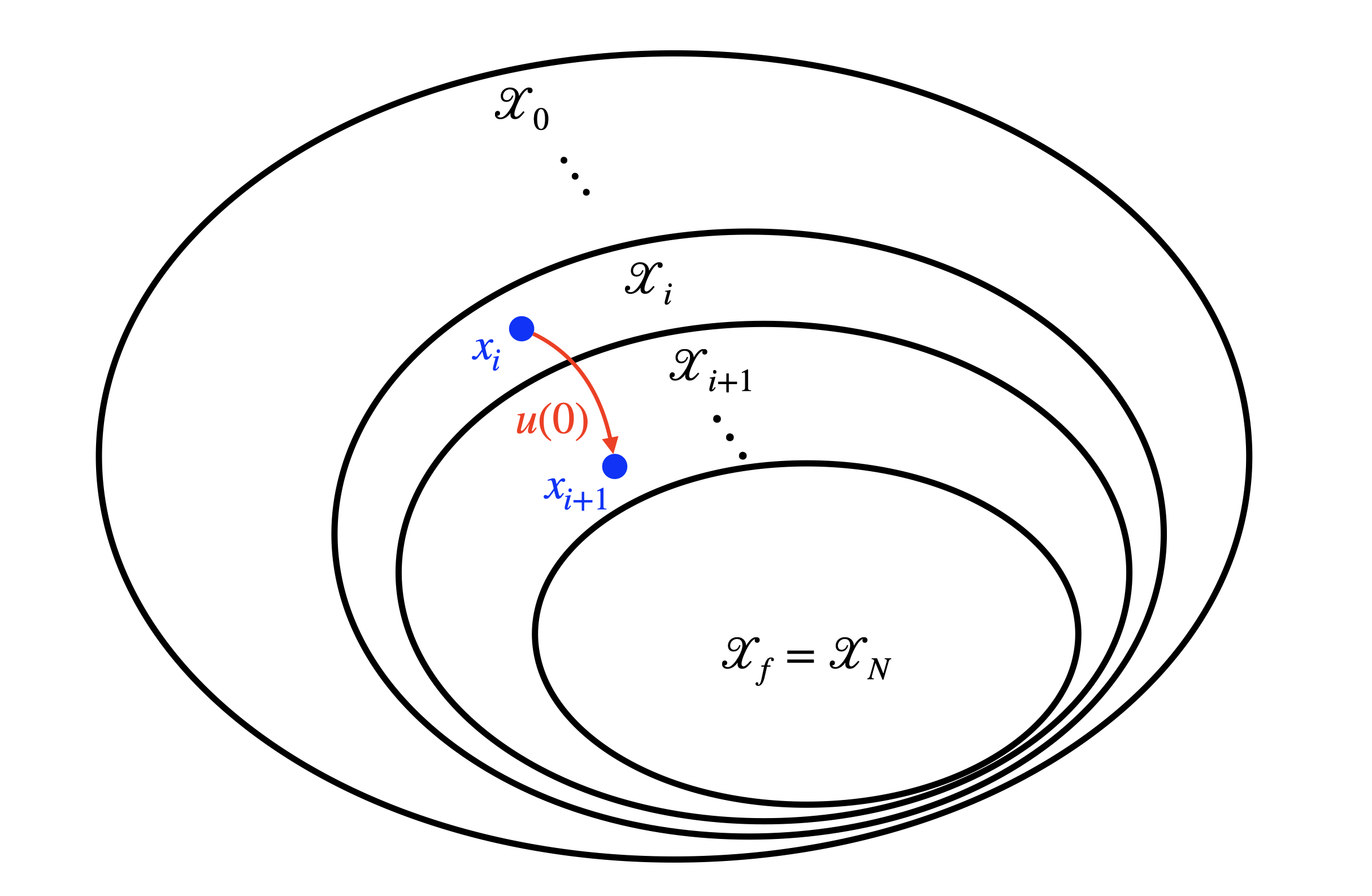
Figure 3.26: Nested control invariant sets.

It suffices to show \(\mathcal{X}_{i+1}\) being control invariant leads to \(\mathcal{X}_i\) being control invariant. First, by \(\mathcal{X}_{i+1}\) control invariant, we have \(\mathcal{X}_{i+1} \subseteq \text{Pre}(\mathcal{X}_i) \cap \mathcal{X} = \mathcal{X}_i\). Now pick any \(x_{i} \in \mathcal{X}_{i}\), for any feasible \(\hat{u}(0),\dots,\hat{u}(N-1)\), applying the first control \(\hat{u}(0)\) brings the system to a new state \[ x_{i+1} = A x_i + B \hat{u}(0) \in \mathcal{X}_{i+1} \subseteq \mathcal{X}_i. \] This shows \(\mathcal{X}_i\) is control invariant.

Persistent feasibility does not guarantee the closed-loop system will converge to the origin. In fact, from Theorem 3.2, it is clear that if the system starts at \(x_0 \in \mathcal{X}_0\), then we can only guarantee \(x_t \in \mathcal{X}_1\) for all \(t \geq 0\).

3.3.5 Stability

We now answer the question of how can we guarantee the RHC controller will drive the system to the desired origin.

Theorem 3.3 (Sufficient Condition for Stability) Consider the linear system (3.33), and the RHC algorithm (3.35). Assume that

1. The stage cost \(q(x,u)\) and terminal cost \(p(x)\) are continuous and positive definite functions.

2. The sets \(\mathcal{X}\), \(\mathcal{X}_f\) and \(\mathcal{U}\) contain the origin in their interior and are closed.

3. \(\mathcal{X}_f \subseteq \mathcal{X}\) is control invariant.

4. For any \(x \in \mathcal{X}_f\), the following inequality holds \[\begin{equation} \min_{u \in \mathcal{U}, A x + Bu \in \mathcal{X}_f} \left( - p(x) + q(x,u) + p(Ax + Bu) \right) \leq 0. \tag{3.40} \end{equation}\]

Then, the origin of the closed-loop system (3.39) is asymptotically stable with domain of attraction \(\mathcal{X}_0\). In words, for any \(x_0 \in \mathcal{X}_0\), if the closed-loop system (3.39) starts at \(x_0\), then the system trajectory converges to the origin as \(t\) tends to infinity.

Let us interpret Theorem 3.3 before proving it. It should be clear that the first three assumptions are easy to satisfy. For example, if we choose \(p(x) = x^T P x\) and \(q(x,u) = x^T Q x + u^T R u\) with \(P, Q, R \succ 0\), then assumption 1 is satisfied. Usually \(\mathcal{X}\) and \(\mathcal{U}\) are both polyhedral sets containing the origin in the interior, so assumption 2 also holds naturally. Finding a control invariant set \(\mathcal{X}_f\) is not a trivial task but there exists numerical algorithms for this task (e.g., using the algorithms introduced in Section 3.3.2.4). After we find a control invariant \(\mathcal{X}_f\), by Theorem 3.2, we know persistent feasibility will hold.

We now prove the theorem by showing that Assumption 4 guarantees stability. Before we show the proof, we need the concept of a Lyapunov function. Below we introduce Lyapunov function for a discrete-time dynamical system, but we will study more details of Lyapunov function for continuous-time dynamical systems in Chapter 5.

Lemma 3.3 (Discrete-time Lyapunov Function) Consider the discrete-time autonomous system (3.27), restated below for convenience: \[ x_{t+1} = f_a(x_t), \] and assume \(x=0\) is an equilibrium point of the system, i.e., \(0 = f_a (0)\) (if the system starts at the origin, it stays at the origin). Let \(\Omega \subset \mathbb{R}^n\) be a closed and bounded set containing the origin. If there exists a function \(V: \mathbb{R}^n \rightarrow \mathbb{R}\) that is (a) continuous at the origin, (b) finite for every \(x \in \Omega\), and (c) satisfies

1. \(V\) is positive definite: \(V(0) = 0\) and \(V(x) > 0,\forall x \in \Omega \backslash \{ 0\}\),

2. \(V(x_{t+1}) - V(x_t) \leq - \alpha(x_t) < 0\) for any \(x_t \in \Omega \backslash \{ 0\}\),

where \(\alpha: \mathbb{R}^n \rightarrow \mathbb{R}\) is a continuous positive definite function. Then \(x=0\) is asymptotically stable in \(\Omega\), i.e, if the system starts within \(\Omega\), then its trajectory tends to \(0\) as \(t \rightarrow \infty\).

A function \(V\) satisfying the conditions above is called a Lyapunov function for the system.

One can think of the Lyapunov function \(V\) as an energy function for the system (3.27) that maps a system state to a single scalar. Condition 1 in Lemma 3.3 states that \(V\) (the energy function) is strictly positive except at the origin. Condition 2 in Lemma 3.3 states that, the system energy \(V\) is strictly decreasing along any system trajectory. Therefore, we conclude that \(V\) must converge to \(V=0\), and hence any state trajectory must converge to the origin.

We will now use Lemma 3.3 to prove RHC stability under Theorem 3.3.

Proof. Our goal is to prove that the optimal cost of the RHC problem (3.35), \(J_t^\star(x_t)\), is a Lyapunov function for the closed-loop system (3.39) on the domain \(\mathcal{X}_0\). Then using Lemma 3.3 we can conclude that the closed-loop system (3.39) will converge to the origin.

Positive definite. Clearly, we have \(J_t^\star(0) = 0\) by the positive definiteness of \(p\) and \(q\) and the fact that \(x=0\) is an equilibrium point of the linear system (3.33). For \(x_t \neq 0\), it is also clear that \(J_t^\star(x) > 0\). Therefore, \(J_t^\star(x)\) is positive definite on \(\mathcal{X}_0\).

Strictly decrease. It suffices to show \(J_1^\star(x_1) - J_0^\star(x_0) < 0\) because the constraints of the RHC problem (3.35) is time-invariant. Pick any \(x_0 \in \mathcal{X}_0\), and let \[\begin{equation} \left( u^\star(0),u^\star(1),\dots,u^\star(N-1) \right) \tag{3.41} \end{equation}\] be an optimal control trajectory to problem (3.35). Denote \[\begin{equation} \left( x_0,x(1),\dots,x(N) \right) \tag{3.42} \end{equation}\] as the associated optimal state trajectory for problem (3.35). The RHC controller will apply \(u^\star(0)\) to the system, leading to the next state \[ x_1 = x(1) = A x_0 + B u^\star(0). \] Then we will solve problem (3.35) to get \(J^\star_1(x_1)\), and we want to show \(J^\star_1(x_1) < J^\star_0(x_0)\). Towards this, we will construct a feasible solution to (3.35) starting at \(x_1\), and hence an upper bound on \(J^\star_1(x_1)\). Consider the control sequence \[\begin{equation} \left( u^\star(1),\dots,u^\star(N-1),v \right) \tag{3.43} \end{equation}\] which is different from the control sequence in (3.41) by removing \(u^\star(0)\) and appending \(v\). The corresponding state trajectory to (3.43) is \[\begin{equation} \left( x_1 = x(1), x(2),\dots,x(N), Ax(N) + Bv \right) \tag{3.44} \end{equation}\] which is different from the state trajectory in (3.42) by removing \(x_0\) and appending \(A x(N) + Bv\). Since \(x(N) \in \mathcal{X}_f\) and \(\mathcal{X}_f\) is control invariant, there exists \(v\) such that \(Ax(N) + Bv \in \mathcal{X}_f\) and the corresponding control trajectory (3.43) is feasible. Applying the control trajectory (3.43) to the optimization problem (3.35) will lead to the total cost \[ J_1(x_1) = J_0^\star(x_0) - q(x_0,u^\star(0)) \underbrace{- p(x(N)) + q(x(N),v) + p(Ax(N) + Bv)}_{s(x(N),v)}. \] Now by assumption 4 in Theorem 3.3, we can choose \(v\) such that the sum \(s(x(N),v) \leq 0\). Consequently, we have \[ J_1^\star(x_1) \leq J_1(x_1) \leq J_0^\star(x_0) - q(x_0,u^\star(0)), \] which leads to \[ J_1^\star(x_1) - J_0^\star(x_0) \leq - q(x_0,u^\star(0)). \] Because the choice of \(x_0\) was arbitrary, we conclude that \(J_t^\star(x_t)\) strictly decreases along any system trajectory that starts within \(\mathcal{X}_0\).

Continuity at the origin. We will show that \(J_0^\star(x) \leq p(x)\) for any \(x \in \mathcal{X}_f\). With this argument, since \(p(x)\) is positive definite and continuous, then \(J_0^\star(x)\) must be continuous at the origin. We now prove \(J_0^\star(x) \leq p(x)\) for any \(x \in \mathcal{X}_f\). Since \(\mathcal{X}_f\) is control invariant, pick any \(x \in \mathcal{X}_f\), there exists a sequence of controls \((u(0),u(1),\dots,u(N-1))\) such that the state trajectory \((x(0)=x,x(1),\dots,x(N))\) stays in \(\mathcal{X}_f\). Such a control sequence lead to an upper bound on \(J^\star_0(x)\): \[ J^\star_0(x(0)) \leq p(x(N)) + \sum_{i=0}^{N-1} q(x(i),u(i)) = p(x(0)) + \sum_{i=0}^{N-1} \left( q(x(i),u(i)) + p(x(i+1)) - p(x(i)) \right), \] since each \(x(i) \in \mathcal{X}_f\), according to Assumption 4, we can choose \(u(i)\) such that \[ J^\star_0(x(0)) \leq p(x(0)) \] for any \(x(0) \in \mathcal{X}_f\).

In conclusion, we have shown that \(J^\star_t(x_t)\) is a Lyapunov function, and by Lemma 3.3, the closed-loop system is asymptotically stable.

A function \(p(x)\) that satisfies Assumption 4 in Theorem 3.3 is typicalled known as a control Lyapunov function.

Now two natural problems arise:

1. Given \(p(x)\), how to verify if assumption 3 holds in Theorem 3.3?

2. How to synthesize a \(p(x)\) that satisfies assumption 3 in Theorem 3.3?

Unfortunately, both problems are hard. To see this, suppose we are given a candidate function \(p(x) = x^T P x\) with \(P \succ 0\) that is clearly positive definite. Assume \(q(x,u) = x^T Q x + u^T R u\) with \(Q, R \succ 0\) and \(\mathcal{U}, \mathcal{X}_f\) are given polyhedral sets. Then verifying if \(p(x)\) satisifies Assumption 4 boils down to checking if \[ \min_{u \in \mathcal{U}, Ax + Bu \in \mathcal{X}_f} x^T Q x + u^T R u + (Ax + Bu)^T P (Ax + Bu) - x^T P x \] is non-positive for any possible \(x \in \mathcal{X}_f\). Although for each possible \(x\), the above problem is a convex optimization problem, there are an infinite number of points in the set \(\mathcal{X}_f\) and enumerating over all points is a daunting task. We will see in Chapter 5 that convex relaxations, in particular semidefinite relaxations, can help us partially solve these hard problems.

A simple control lyapunov function. One can solve the infinite-horizon unconstrained LQR problem \[ \min_{u_t} \sum_{t=0}^{\infty}x_t ^T Q x_t + u_t^T R u_t, \] for which the optimal cost-to-go is \[ J_{\infty}(x) = x^T S x, \] with \(S\) the solution to the algebraic Riccati equation (2.13). Denote \[ u_t = \Pi_{\mathcal{U}} (- K x_t) \] as the optimal controller (\(\Pi_{\mathcal{U}}\) is the projection of the controller to the feasible set \(\mathcal{U}\)), and use \(\mathcal{X}_f\) as the maximal positive invariant set of the closed-loop system \[ x_{t+1} = A x_t + B u_t. \] Then \(J_{\infty}(x) = x^T S x\) is a control Lyapunov function over the set \(\mathcal{X}_f\).

3.3.6 Explicit MPC

See the original paper (Bemporad et al. 2002), and check out Matlab’s explict MPC design.

3.4 Policy Gradient

References

Bemporad, Alberto, Manfred Morari, Vivek Dua, and Efstratios N Pistikopoulos. 2002. “The Explicit Linear Quadratic Regulator for Constrained Systems.” Automatica 38 (1): 3–20.

Bertsekas, Dimitri. 1972. “Infinite Time Reachability of State-Space Regions by Using Feedback Control.” IEEE Transactions on Automatic Control 17 (5): 604–13.

Borrelli, Francesco, Alberto Bemporad, and Manfred Morari. 2017. Predictive Control for Linear and Hybrid Systems. Cambridge University Press.

Gilbert, Elmer G, and K Tin Tan. 1991. “Linear Systems with State and Control Constraints: The Theory and Application of Maximal Output Admissible Sets.” IEEE Transactions on Automatic Control 36 (9): 1008–20.

Kelly, Matthew. 2017. “An Introduction to Trajectory Optimization: How to Do Your Own Direct Collocation.” SIAM Review 59 (4): 849–904.

Kolmanovsky, Ilya, Elmer G Gilbert, et al. 1998. “Theory and Computation of Disturbance Invariant Sets for Discrete-Time Linear Systems.” Mathematical Problems in Engineering 4: 317–67.

Levine, Nir, Tom Zahavy, Daniel J Mankowitz, Aviv Tamar, and Shie Mannor. 2017. “Shallow Updates for Deep Reinforcement Learning.” Advances in Neural Information Processing Systems 30.

Mnih, Volodymyr, Koray Kavukcuoglu, David Silver, Andrei A Rusu, Joel Veness, Marc G Bellemare, Alex Graves, et al. 2015. “Human-Level Control Through Deep Reinforcement Learning.” Nature 518 (7540): 529–33.

Nocedal, Jorge, and Stephen J Wright. 1999. Numerical Optimization. Springer.

Yang, Alan, and Stephen Boyd. 2023. “Value-Gradient Iteration with Quadratic Approximate Value Functions.” arXiv Preprint arXiv:2307.07086.