Chapter 4 Continuous-time Optimal Control
So far we have been focusing on stochastic and discrete-time optimal control problems. In this Chapter, we will switch gear to deterministic and continuous-time optimal control (still with continuous state and action space).
The goal of a continuous-time introduction is threefold. (1) Real-world systems are natively continuous-time. (2) We will see the continuous-time analog of the Bellman principle of optimality in discrete-time (cf. Theorem 1.1). (3) The continuous-time setup is more natural and popular for stability analysis to be introduced in Chapter 5.
4.1 The Basic Problem
Consider a continuous-time dynamical system \[\begin{equation} \dot{x}(t) = f(x(t),u(t)),\ t \in [0,T], \quad x(0) = x_0, \tag{4.1} \end{equation}\] where
\(x(t) \in \mathbb{R}^n\) is the state of the system,
\(u(t) \in \mathbb{U} \subseteq \mathbb{R}^m\) is the control we wish to design,
\(f: \mathbb{R}^{n} \times \mathbb{R}^m \rightarrow \mathbb{R}^n\) models the system dynamics, and
\(x_0 \in \mathbb{R}^n\) is the initial state of the system.
We assume the admissible control functions \(\{u(t) \mid u(t) \in \mathbb{U}, t\in [0,T] \}\), also called control trajectories, must be piecewise continuous.4 For any control trajectory, we assume the system (4.1) has a unique solution \(\{x(t)\mid t \in [0,T] \}\), called the state trajectory.
We now state the continuous-time optimal control problem.
Definition 4.1 (Continuous-time, Finite-horizon Optimal Control) Find the best admissible control trajectory \(\{u(t) \mid t \in [0,T] \}\) that minimizes the cost function \[\begin{equation} J(0,x_0) = \min_{u(t) \in \mathbb{U}} h(x(T)) + \int_0^T g(x(t),u(t)) dt, \tag{4.2} \end{equation}\] subject to (4.1), where the functions \(g\) and \(h\) are continuously differentiable with respect to \(x\), and \(g\) is continuous with respect to \(u\).
The function \(J\) in (4.2) is called the optimal cost-to-go, or the optimal value function. Notice that the optimal cost-to-go is a function of both the state \(x\) and the time \(t\), just as in the discrete-time case we used \(J_k\) with a subscript \(k\) to denote the optimal cost-to-go for the tail problem starting at timestep \(k\) (cf. Theorem 1.2). Specifically, we should interpret \[ J(t,x_0) = \min_{u(t) \in \mathbb{U}} h(x(T)) + \int_t^T g(x(\tau),u(\tau)) d\tau, \quad x(t) = x_0, \] as the optimal cost-to-go of the system starting from \(x_0\) at time \(t\) (i.e., the tail problem). We assume \(J(0,x_0)\) is finite when \(x_0\) is in some set \(\mathcal{X}_0\).
4.2 The Hamilton-Jacobi-Bellman Equation
Recall that in discrete-time, the dynamic programming (DP) algorithm in Theorem 1.2 states that the optimal cost-to-go has to satisfy a recursive equation (1.5), i.e., the optimal cost-to-go at time \(k\) can be calculated by choosing the best action that minimizes the stage cost at time \(k\) plus the optimal cost-to-go at time \(k+1\). In the next, we will show a result of similar flavor to (1.5), but in the form of a partial differential equation (PDE), known as the Hamilton-Jacobi-Bellman (HJB) equation.
Let us informally derive the HJB equation by applying the DP algorithm to a discrete-time approximation of the continuous-time optimal control problem. We divide the time horizon \([0,T]\) into \(N\) pieces of equal length \(\delta = T/N\), and denote \[ x_k = x(k\delta), \quad u_k = u(k \delta), \quad k = 0,1,\dots,N. \] We then approximate the continuous-time dynamics (4.1) as \[ x_{k+1} = x_k + \dot{x}_k \cdot \delta = x_k + f(x_k,u_k) \cdot \delta, \] and the cost function in (4.2) as \[ h(x_N) + \sum_{k=0}^{N-1} g(x_k, u_k)\cdot \delta. \] This problem now is in the form of a discrete-time, finite-horizon optimal control 1.1, for which we can apply dynamic programming.
Let us use \(\tilde{J}(t,x)\) (as opposed to \(J(t,x)\)) to denote the optimal cost-to-go at time \(t\) and state \(x\) for the discrete-time approximation. According to (1.5), the DP backward recursion is \[\begin{align} \tilde{J}(N\delta,x) = h(x), \\ \tilde{J}(k\delta,x) = \min_{u \in \mathbb{U}} \left[ g(x,u)\cdot \delta + \tilde{J}((k+1)\delta,x + f(x,u)\cdot \delta) \right], \quad k = N-1,\dots,0. \tag{4.3} \end{align}\] Suppose \(\tilde{J}(t,x)\) is differentiable, we can perform a Taylor-series expansion of \(\tilde{J}((k+1)\delta,x+f(x,u)\delta)\) in (4.3) as follows \[ \tilde{J}((k+1)\delta,x+f(x,u)\delta) = \tilde{J}(k\delta,x) + \nabla_t \tilde{J} (k\delta,x) \cdot \delta + \nabla_x \tilde{J}(k\delta,x)^T f(x,u) \cdot \delta + o(\delta), \] where \(o(\delta)\) includes high-order terms that approach zero when \(\delta\) tends to zero, \(\nabla_t \tilde{J}\) and \(\nabla_x \tilde{J}\) (a column vector) denote the partial derivates of \(\tilde{J}\) with respect to \(t\) and \(x\), respectively. Plugging the first-order Taylor expansion into the DP recursion (4.3), we obtain \[\begin{equation} \tilde{J}(k\delta,x) = \min_{u \in \mathbb{U}} \left[ g(x,u) \cdot \delta + \tilde{J}(k \delta,x) + \nabla_t \tilde{J}(k \delta,x) \delta + \nabla_x \tilde{J}(k\delta,x)^T f(x,u) \delta + o(\delta) \right]. \tag{4.4} \end{equation}\] Cancelling \(\tilde{J}(k \delta,x)\) from both sides, dividing both sides by \(\delta\), and assuming \(\tilde{J}\) converges to \(J\) uniformly in time and state, i.e., \[ \lim_{\delta \rightarrow 0, k\delta = t} \tilde{J}(k\delta,x) = J(t,x), \quad \forall t,x, \] we obtain from (4.4) the following partial differential equation \[\begin{equation} 0 = \min_{u \in \mathbb{U}} \left[ g(x,u) + \nabla_t J(t,x) + \nabla_x J(t,x)^T f(x,u) \right], \quad \forall t, x, \tag{4.5} \end{equation}\] with the boundary condition \(J(T,x) = h(x)\). Equation (4.5) is called the Hamilton-Jacobi-Bellman equation.
Our derivation above is informal, let us formally state the HJB equation.
Theorem 4.1 (Hamilton-Jacobi-Bellman Equation as A Sufficient Condition for Optimality) Consider the optimal control problem 4.1 for system (4.1). Suppose \(V(t,x)\) is a solution to the Hamilton-Jacobi-Bellman equation, i.e., \(V(t,x)\) is continuously differentiable and satisfies \[\begin{align} \tag{4.6} 0 = \min_{u \in \mathbb{U}} \left[ g(x,u) + \nabla_t V(t,x) + \nabla_x V(t,x)^T f(x,u)\right], \quad \forall t,x, \\ V(T,x) = h(x), \quad \forall x. \end{align}\] Suppose \(\mu^\star(t,x)\) attains the minimum in (4.6) for all \(t\) and \(x\). Let \(\{x^\star(t) \mid t \in [0,T] \}\) be the state trajectory obtained from the given initial condition \(x(0)\) when the control trajectory \(u^\star(t) = \mu^\star(t,x^\star(t))\) is applied, i.e., \(x^\star(0) = x(0)\) and for any \(t \in [0,T]\), \(\dot{x}^\star(t) = f(x^\star(t), \mu^\star(t,x^\star(t)))\) and we assume this differential equation has a unique solution starting at any \((t,x)\) and that the control trajectory \(\{ \mu^\star(t,x^\star(t)) \mid t \in [0,T] \}\) is piecewise continuous as a function of \(t\). Then \(V(t,x)\) is equal to the optimal cost-to-go \(J(t,x)\) for all \(t\) and \(x\). Moreover, the control trajectory \(u^\star(t)\) is optimal.
Proof. Let \(\{\hat{u}(t) \mid t \in [0,T] \}\) be any admissible control trajectory and let \(\hat{x}(t)\) be the resulting state trajectory. From the “\(\min\)” in (4.6), we know \[ 0 \leq g(\hat{x},\hat{u}) + \nabla_t V(t,\hat{x}) + \nabla_x V(t,\hat{x})^T f(\hat{x},\hat{u}) = g(\hat{x},\hat{u}) + \frac{d}{dt} V(t,\hat{x}). \] Integrating the above inequality over \(t \in [0,T]\), we obtain \[ 0 \leq \left( \int_{0}^T g(\hat{x}(t),\hat{u}(t))dt \right) + V(T,\hat{x}(T)) - V(0,\hat{x}(0)). \] Using the terminal constraint \(V(T,x) = h(x)\) for any \(x\) and the initial condition \(\hat{x}(0) = x(0)\), we have \[ V(0,x(0)) \leq h(\hat{x}(T)) + \int_{0}^T g(\hat{x}(t),\hat{u}(t)) dt. \] This shows that \(V(0,x(0))\) is a lower bound to the optimal cost-to-go, because any admissible control trajectory \(\hat{u}(t)\) leads to a cost no smaller than \(V(0,x(0))\).
It remains to show that \(V(0,x(0))\) is attainable. This is done by plugging the optimal control trajectory \(u^\star(t)\) and state trajectory \(x^\star(t)\) to the derivation above, leading to \[ V(0,x(0)) = h(x^\star(T)) + \int_0^T g(x^\star(t),u^\star(t)) dt. \] This shows that \(V(0,x(0)) = J(0,x(0))\).
The argument above is generic and holds for any initial time \(t \in [0,T]\) and initial state \(x\). Therefore, \(V(t,x) = J(t,x)\) is the optimal cost-to-go.
Theorem 4.1 effectively turns the optimal control problem (4.2) into finding a solution for the partial differential equation (4.6). Let us illustrate the theorem using a simple example.
Example 4.1 (A Scalar System) Consider the following dynamical system \[ \dot{x}(t) = u(t), \quad t \in [0,T] \] where \(x \in \mathbb{R}\) is the state, and \(u \in \mathbb{U} = [-1,1]\) is the control.
We are interested in the following optimal control problem \[ \min_{u(t)} \frac{1}{2} \left( x(T) \right)^2, \] where the goal is to move the initial state as close as possible to the origin \(0\) at the terminal time \(T\).
There is a simple optimal controller for this scalar system. We move the state as quickly as possible to the origin \(0\), using maximum control, and then maintain the state at the origin using zero control. Formally, this is \[ \mu^\star(t,x) = - \text{sgn}(x) = \begin{cases} 1 & \text{if } x < 0 \\ 0 & \text{if } x = 0 \\ -1 & \text{if } x > 0 \end{cases}. \] With this controller, we know that if the system starts at \(x\) at time \(t\), the terminal state will satisfy \[ \vert x(T) \vert = \begin{cases} |x| - (T - t) & \text{if } T-t < |x| \\ 0 & \text{otherwise} \end{cases}. \] As a result, the optimal cost-to-go is \[\begin{equation} J(t,x) = \frac{1}{2} \left( \max\{0, |x| - (T - t)\} \right)^2. \tag{4.7} \end{equation}\]
Let us verify if this function satisfies the HJB equation.
Boundary condition. Clearly, \[ J(T,x) = \frac{1}{2}x^2 \] satisfies the boundary condition.
Differentiability. When viewed as a function of \(t\), \(J(t,x)\) in (4.7) can be plotted as in Fig. 4.1. We can see that \(J(t,x)\) is differentiable in \(t\) and \[\begin{equation} \nabla_t J(t,x) = \max\{ 0, |x| - (T-t) \}. \tag{4.8} \end{equation}\]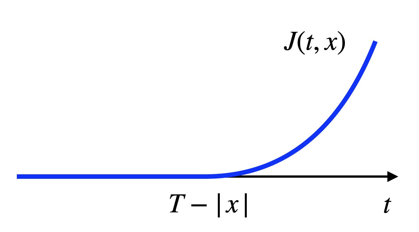
Figure 4.1: Optimal cost-to-go as a function of time.
When viewed as a function of \(x\), \(J(t,x)\) can be plotted as in Fig. 4.2. We can see \(J(t,x)\) is differentiable in \(x\) and \[\begin{equation} \nabla_x J(t,x) = \text{sgn}(x) \cdot \max\{ 0,|x| - (T-t) \}. \tag{4.9} \end{equation}\]
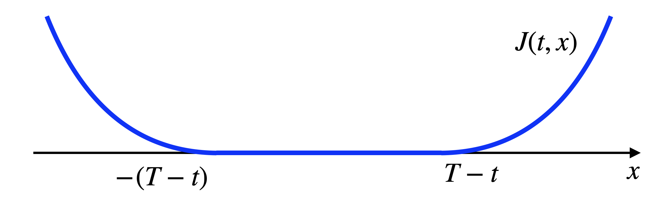
Figure 4.2: Optimal cost-to-go as a function of state.
PDE. Substituting (4.8) and (4.9) into the HJB equation (4.6), we need to verify that the followng equation holds for all \(t\) and \(x\) \[\begin{equation} 0 = \min_{u \in \mathbb{U}} (1 + \text{sgn}(x) \cdot u) \max\{0, |x| - (T-t) \}. \tag{4.10} \end{equation}\] This is easy to verify as \(u = - \text{sgn}(x)\) attains the minimum and sets the right-hand side equal to zero for any \((t,x)\).
However, we can observe that the optimal controller need not be unique. For example, when \(|x| \leq T-t\), we have \[ \max\{0, |x| - (T-t) \} = 0, \] and any \(u \in \mathbb{U}\) would attain the minimum in (4.10) and hence be optimal.
For simple systems, the HJB equation can be solved numerically.
Example 4.2 (Numerical HJB Solution of A Scalar System) Consider a scalar linear system \[ \dot{x} = x + u, \] and the optimal control problem with quadratic costs and \(T=0.5\) \[ \min_{u(t),t\in[0,T]} x(T)^T P x(T) + \int_{t=0}^T (x^T Q x + u^T R u ) dt \] with \(P=Q=R=1\). Solve the HJB equation on a mesh \(x \in [-8,8]\), we obtain the optimal cost-to-go in Fig. 4.3.
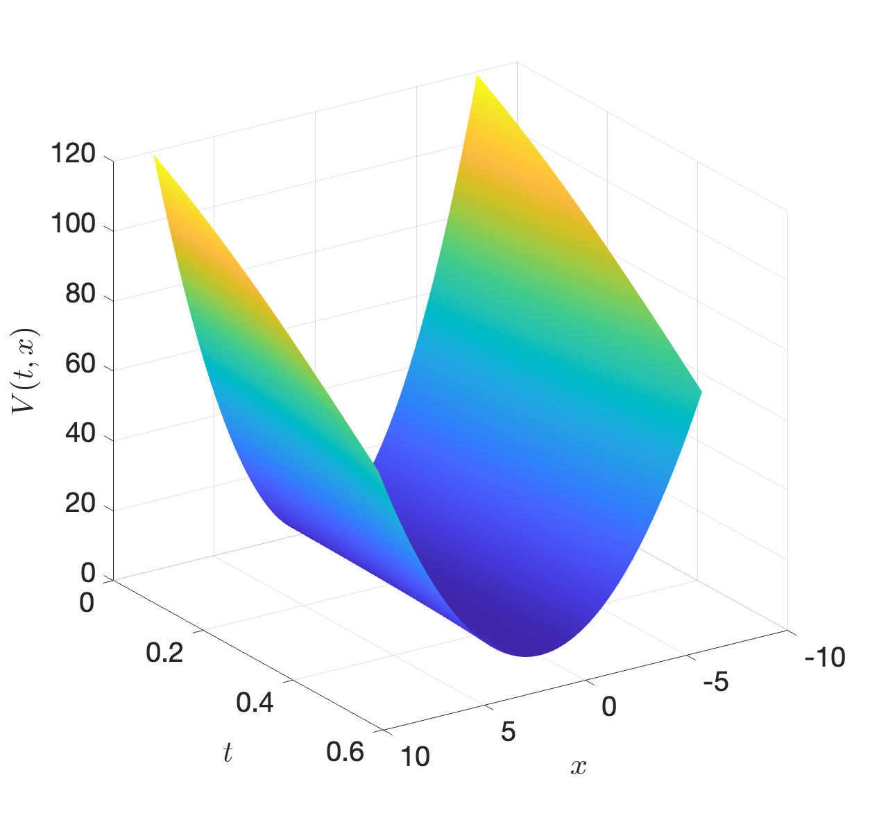
Figure 4.3: Numerical solution of the HJB equation.
You can find code for this problem here.
4.3 Linear Quadratic Regulator
Let us apply the HJB sufficiency Theorem 4.1 to the continuous-time linear quadratic regulator (LQR).
Consider the linear system \[ \dot{x}(t) = A x(t) + B u(t), \] with \(x \in \mathbb{R}^n\), \(u \in \mathbb{R}^m\), and the optimal control problem \[ \min_{u(t),t\in [0,T]} x(T)^T P x(T) + \int_{t=0}^T (x(t)^T Q x(t) + u(t)^T R u(t)) dt \] where \(P,Q\succeq 0\) and \(R \succ 0\).
According to Theorem 4.1, the HJB equation for this problem is \[\begin{equation} \begin{split} 0 = \min_{u \in \mathbb{R}^m } \left[ x^T Q x + u^T R u + \nabla_t V(t,x) + \nabla_x V(t,x)^T f(x,u) \right], \quad \forall t,x, \\ V(T,x) = x^T P x, \quad \forall x. \end{split} \tag{4.11} \end{equation}\]
Let us guess a solution of the following form, \[ V(t,x) = x^T S(t) x, \quad S(t) \in \mathbb{S}^n, \] where \(\mathbb{S}^n\) is the set of \(n \times n\) symmetric matrices.
The second equation in the HJB (4.11) implies \[\begin{equation} S(T) = P. \tag{4.12} \end{equation}\] The first equation in the HJB (4.11) requires \[\begin{equation} 0 = \min_{u \in \mathbb{R}^m} \left[ x^T Q x + u^T R u + x^T \dot{S}(t) x + 2x^T S(t) (A x + Bu) \right]. \tag{4.13} \end{equation}\] The objective function to be minimized in (4.13) is a convex quadratic function of \(u\), hence the optimal solution satisfies \[ 2 R u^\star + 2B^T S(t) x = 0, \] solving which yields \[\begin{equation} u^\star = - R^{-1} B^T S(t) x. \tag{4.14} \end{equation}\] Now plugging the solution (4.14) back into (4.13), we obtain \[ 0 = x^T \left[ \dot{S}(t) + S(t) A + A^T S(t) - S(t)B R^{-1} B^T S(t) + Q \right] x, \quad \forall (t,x), \] which implies that \(\dot{S}(t)\) must satisfy \[\begin{equation} \dot{S}(t) = - S(t) A - A^T S(t) + S(t) B R^{-1} B^T S(t) - Q. \tag{4.15} \end{equation}\] This is known as the continuous-time differential Riccati equation, with the terminal condition given in (4.12). You should compare (4.15) with its discrete-time counterpart (2.7) and observable their similarities.
4.3.1 LQR Trajectory Tracking
So far we have been talking about LQR in the context of regulating the system to a desired equilibrium point (usually the origin), you can in fact also use LQR for tracking a reference trajectory.
Consider again the linear system \[ \dot{x}(t) = A x (t) + B u(t), \quad x \in \mathbb{R}^n, u \in \mathbb{R}^m. \] Given a reference state-control trajectory \((x_r(t),u_r(t))_{t \in [0,T]}\), we consider the following optimal control problem to track the reference trajectory \[ \min_{u(t),t \in [0,T]} \Vert x(T) - x_r(T) \Vert_P^2 + \int_{t=0}^T \left( \Vert x(t) - x_r(t) \Vert_Q^2 + \Vert u(t) - u_r(t) \Vert_R^2 \right) dt \] where \(\Vert v \Vert_A^2 := v^T A v\), \(P,Q\succeq 0\) and \(R \succ 0\).
Let us guess a solution to the HJB of the following form \[ V(t,x) = x^T S_{xx}(t) x + 2 x^T s_x(t) + s_0(t) = \begin{bmatrix} x \\ 1 \end{bmatrix}^T \underbrace{\begin{bmatrix} S_{xx}(t) & s_x(t) \\ s_x^T(t) & s_0(t) \end{bmatrix}}_{=: S(t)} \begin{bmatrix} x \\ 1 \end{bmatrix}, \quad S(t) \succ 0. \] Differentiating \(V(t,x)\) with respect to \(t\) and \(x\) we obtain \[\begin{equation} \begin{split} \nabla_t V(t,x) = x^T \dot{S}_{xx}(t) x + 2 x^T \dot{s}_x(t) + \dot{s}_0(t), \\ \nabla_x V(t,x) = 2 S_{xx}(t) x + 2 s_x(t). \end{split} \end{equation}\] Plugging the partial derivates into the HJB (4.6), we have \[ 0 = \min_{u} \left[ \Vert x - x_r \Vert_Q^2 + \Vert u - u_r \Vert_R^2 + \nabla_x V(t,x)^T (A x + Bu) + \nabla_t V(t,x) \right]. \] The objective to be minimized is convex in \(u\), leading to a closed-form solution \[\begin{equation} u^{\star}(t) = u_r(t) - R^{-1}B^T \left[ S_{xx}(t)x + s_x(t) \right]. \tag{4.16} \end{equation}\] With the solution of \(u\) (4.16) plugged back into the HJB, we can find the differential equations that \(S_{xx}(t)\), \(s_x(t)\) and \(s_0(t)\) need to satisfy \[\begin{equation} \begin{split} -\dot{S}_{xx}(t) = Q - S_{xx}(t) B R^{-1} B^T S_{xx}(t) + S_{xx}(t)A + A^T S_{xx}(t) \\ - \dot{s}_x(t) = -Q x_r(t) + [A^T - S_{xx}(t)B R^{-1} B^T]s_x(t) + S_{xx}(t) B u_r(t) \\ - \dot{s}_0(t) = x_r(t)^T Q x_r(t) - s_x^T(t) B R^{-1} B^T s_x(t) + 2 s_x(t)^T B u_r(t), \end{split} \tag{4.17} \end{equation}\] with the terminal conditions \[\begin{equation} \begin{split} S_{xx}(T) = P \\ s_x(T) = - P x_r(T) \\ s_0(T) = x_r^T(T) P x_r(T). \end{split} \end{equation}\] Notice that the differential equation of \(S_{xx}(t)\) in (4.17) is the same as the differential equation in (4.15). Also notice the value of \(s_0(t)\) does not affect the optimal control (4.16) and hence can often be ignored.
4.3.2 LQR Trajectory Stabilization
Recall that in Example 3.8, we have seen the failure of directly applying open-loop control obtained from trajectory optimization. We then used receding horizon control to turn open-loop trajectory optimization into a close-loop controller.
Another way to stabilize the open-loop trajectory is to perform local LQR stabilization.
Given the nonlinear system \[ \dot{x} = f(x,u), \] suppose we have computed a nominal state-control reference trajectory \((x_r(t),u_r(t))_{t \in [0,T]}\) (e.g., using trajectory optimization), then we can define a local coordinate system relative to the reference trajectory \[ \bar{x}(t) = x(t) - x_r(t), \quad \bar{u}(t) = u(t) - u_r(t). \] The \(\bar{x}\) coordinate satisfies the following dynamics \[\begin{equation} \dot{\bar{x}} = \dot{x} - \dot{x}_r = f(x,u) - f(x_r, u_r). \tag{4.18} \end{equation}\] We can perform a Taylor expansion of the dynamics in (4.18) \[\begin{equation} \hspace{-10mm} \dot{\bar{x}} \approx f(x_r, u_r) + \frac{\partial f(x_r,u_r)}{\partial x} (x - x_r) + \frac{\partial f(x_r,u_r)}{\partial u} (u - u_r) - f(x_r, u_r) = A(t) \bar{x} + B(t) \bar{u}, \tag{4.19} \end{equation}\] where \[ A(t) = \frac{\partial f(x_r(t),u_r(t))}{\partial x}, \quad B(t) = \frac{\partial f(x_r(t),u_r(t))}{\partial u}, \] are time-varying linear matrices.
We then formulate the LQR problem for the approximate linear time-varying system (4.19) \[\begin{equation} \min_{\bar{u}(t), t \in [0,T]} \bar{x}(T)^T P \bar{x}(T) + \int_{t=0}^T \left( \bar{x}(t)^T Q \bar{x}(t) + \bar{u}(t)^T R \bar{u}(t) \right) dt \tag{4.20} \end{equation}\] with \(P \succeq 0, Q \succeq 0, R \succ 0\). The solution to (4.20), according to (4.14) is \[ \bar{u}(t) = - R^{-1} B^T S(t) \bar{x}, \] which implies \[\begin{equation} u(t) = u_r(t) - R^{-1} B^T S(t) (x(t) - x_r(t)) \tag{4.21} \end{equation}\] in the original coordinates. Note that the controller in (4.21) is a feedback controller that “finetunes” the open-loop control.
4.4 The Pontryagin Minimum Principle
The HJB equation in Theorem 4.1 provides a sufficient condition for the optimal cost-to-go. However, since the HJB equation is a sufficient condition, there do exist cases where the optimal cost-to-go does not satisfy the HJB equation but is still optimal (e.g., when the optimal cost-to-go is not continuously differentiable).
We now introduce a necessary condition that any optimal control trajectory and state trajectory must satisfy. This condition is the celebrated Pontryagin minimum principle.
A rigorous derivation of the Pontryagin minimum principle can be mathematically involving and is beyond the scope of this lecture notes (see Section 7.3.2 in (Bertsekas 2012) for a more rigorous treatment). In the following, we provide an informal derivation of the Pontryagin minimum principle.
Recall the HJB equation in Theorem 4.1 states that, if a control trajectory \(u^\star(t)\) and the associated state trajectory \(x^\star(t)\) is optimal, then for all \(t \in [0,T]\), the following condition must hold \[\begin{equation} u^\star(t) = \arg\min_{u \in \mathbb{U}} \left[ g(x^\star(t),u) + \nabla_x J(t,x^\star(t))^T f(x^\star(t),u) \right] \tag{4.22}. \end{equation}\] The above equation says, in order to compute the optimal control, we do not need to know the value of \(\nabla_x J\) at all possible values of \(x\) and \(t\) (which is what the HJB equation tries to do), and we only need to know the value of \(\nabla_x J\) along the optimal trajectory, i.e., to know only \(\nabla_x J(t,x^\star(t))\).
The Pontryagin minimum principle builds upon this key observation, and it points out that \(\nabla_x J(t,x^\star(t))\) (but not \(\nabla_x J(t,x)\) for any \(x\)) satisfies a certain differential equation called the adjoint equation.
We now provide an informal derivation of the adjoint equation that is based on differentiating the HJB equation. Towards this goal, we first present the following lemma which is itself quite useful.
Lemma 4.1 (Differentiating Functions Involving Minimization) Let \(F(t,x,u)\) be a continuously differentiable function of \(t \in \mathbb{R}\), \(x \in \mathbb{R}^n\), \(u \in \mathbb{R}^m\), and let \(\mathbb{U}\) be a convex subset of \(\mathbb{R}^m\). Suppose \(\mu^\star(t,x)\) is a continuously differentiable function such that \[ \mu^\star(t,x) = \arg\min_{u \in \mathbb{U}} F(t,x,u), \quad \forall t,x. \] Then \[\begin{align} \nabla_t \left\{ \min_{u \in \mathbb{U}} F(t,x,u) \right\} = \nabla_t F(t,x,\mu^\star(t,x)), \quad \forall t,x, \\ \nabla_x \left\{ \min_{u \in \mathbb{U}} F(t,x,u) \right\} = \nabla_x F(t,x,\mu^\star(t,x)), \quad \forall t,x. \end{align}\] In words, the partial derivates (with respect to \(t\) and \(x\)) of “the minimum of \(F(t,x,u)\) over \(u\)” (commonly known in optimization as the value function \(\psi(t,x)\) of \(F(t,x,u)\)) are equal to the partial derivates of \(F(t,x,u)\) (with respect to \(t\) and \(x\)) after plugging in the optimizer \(\mu^\star(t,x)\).
We now start with the HJB equation in (4.6), restated below with \(V(t,x)\) replaced by the optimal \(J(t,x)\) for the reader’s convenience \[\begin{equation} 0 = \min_{u \in \mathbb{U}} \left[ g(x,u) + \nabla_t J(t,x) + \nabla_x J(t,x)^Tf(x,u) \right]. \tag{4.23} \end{equation}\] Assume that \(\mu^\star(t,x)\) attains the minimum in the equation above and it is also continuously differentiable. Note that we have made the restrictive assumption that \(\mathbb{U}\) is convex and \(\mu^\star(t,x)\) is continuously differentiable, which are not necessary in a more rigorous derivation of Pontryagin’s principle (cf. Section 7.3.2 in (Bertsekas 2012)).
We differentiate both sides of (4.23) with respect to \(t\) and \(x\). In particular, let \[ F(t,x,u) = g(x,u) + \nabla_t J(t,x) + \nabla_x J(t,x)^T f(x,u) \] and invoke Lemma 4.1, we can write \[\begin{align} \tag{4.24} \hspace{-12mm} 0 = \nabla_x g(x, \mu^\star(t,x)) + \nabla^2_{xt} J(t,x) + \nabla^2_{xx} J(t,x)f(x,\mu^\star(t,x)) + \nabla_x f(x,\mu^\star(t,x)) \nabla_x J(t,x).\\ \hspace{-12mm} 0 = \nabla^2_{tt}J(t,x) + \nabla_{xt}^2 J(t,x)^T f(x,\mu^\star(t,x)) \tag{4.25} \end{align}\] where the first equation results from differentiation of (4.23) with respect to \(x\), and the second equation results from differentiation of (4.23) with respect to \(t\). In (4.24), \(\nabla_x f(x,\mu^\star(t,x))\) is \[ \nabla_f = \begin{bmatrix} \frac{\partial f_1}{\partial x_1} & \cdots & \frac{\partial f_n}{x_1} \\ \vdots & \ddots & \vdots \\ \frac{\partial f_1}{\partial x_n} & \cdots & \frac{\partial f_n}{\partial x_n} \end{bmatrix} \] evaluated at \((x,\mu^\star(t,x))\). Equations (4.24) and (4.25) hold for any \((t,x)\) (under the restrictive assumptions we have made).
We then evaluate the equations (4.24) and (4.25) only along the optimal control and state trajectory \((u^\star(t),x^\star(t))\) that satisfies \[\begin{equation} \dot{x}^\star(t) = f(x^\star(t),u^\star(t)), \quad u^\star(t) = \mu^\star(t,x^\star(t)), \quad t \in [0,T]. \tag{4.26} \end{equation}\] Specifically, along the optimal trajectory, we have \[ \frac{d}{dt} \left( \nabla_x J(t,x^\star(t)) \right) = \nabla^2_{xt} J(t,x^\star(t)) + \nabla^2_{xx} J(t,x^\star(t))f(x^\star(t),u^\star(t)), \] where the right-hand side contains terms in the right-hand side of (4.24) (when evaluted along the optimal trajectory). Similarly, \[ \frac{d}{dt} \left( \nabla_t J(t,x^\star(t)) \right) = \nabla^2_{tt} J(t,x^\star(t)) + \nabla^2_{xt} J(t,x^\star(t))^T f(x^\star(t),u^\star(t)), \] where the right-hand side is exactly the right-hand side of (4.25) (when evaluted along the optimal trajectory). As a result, equations (4.24) and (4.25), when evaluated along the optimal trajectory, are equivalent to \[\begin{align} \tag{4.27} 0 = \nabla_x g(x^\star(t), u^\star(t)) + \frac{d}{dt}\left( \nabla_x J(t,x^\star(t)) \right) + \nabla_x f(x^\star(t),u^\star(t)) \nabla_x J(t,x^\star(t)).\\ 0 = \frac{d}{dt}\left( \nabla_t J(t,x^\star(t)) \right). \tag{4.28} \end{align}\] Therefore, if we denote \[ p(t) = \nabla_x J(t,x^\star(t)), \quad p_0(t) = \nabla_t J(t,x^\star(t)), \] then equations (4.27) and (4.28) become \[\begin{align} \tag{4.29} \dot{p}(t) = - \nabla_x f(x^\star(t),u^\star(t)) p(t) - \nabla_x g(x^\star(t),u^\star(t)), \\ \dot{p}_0(t) = 0. \tag{4.30} \end{align}\] Equation (4.29), which is a system of \(n\) first-order differential equations, is known as the adjoint equation and it describes the evolution of \(p(t)\), known as the costate, along the optimal trajectory. To obtain a boundary condition for the adjoint equation (4.29), we note that the boundary condition of the HJB equation \[ J(T,x) = h(x),\quad \forall x \] implies \[ p(T) = \nabla h(x^\star(T)). \]
This is basically the Pontryagin Minimum Principle.
The Hamiltonian formulation. It is usually more convenient to state the Pontryagin Principle using the concept of a Hamiltonian. Formally, we define the Hamiltonian function that maps the triplet \((x,u,p) \in \mathbb{R}^n \times \mathbb{R}^m \times \mathbb{R}^n\) to real numbers given by \[ H(x,u,p) = g(x,u) + p^T f(x,u). \] Note that the dynamics along the optimal trajectory (4.26) can be conveniently written as \[ \dot{x}^\star(t) = \nabla_p H(x^\star(t),u^\star(t),p(t)), \] and the adjoint equation (4.29) can be written as \[ \dot{p}(t) = - \nabla_x H(x^\star(t), u^\star(t), p(t)). \] We are now ready to state the Pontryagin Minimum Principle.
Theorem 4.2 (Pontryagin Minimum Principle as A Necessary Condition for Optimality) Let \((u^\star(t), x^\star(t)), t \in [0,T]\) be a pair of optimal control and state trajectories satisfying \[ \dot{x}^\star(t) = f(x^\star(t),u^\star(t)), \quad x^\star(0) = x_0 \text{ given}. \] Let \(p(t)\) be the solution of the adjoint equation \[ \dot{p}(t) = - \nabla_x H(x^\star(t),u^\star(t),p(t)), \] with the boundary condition \[ p(T) = \nabla h(x^\star(T)), \] where \(h\) is the terminal cost function. Then, for all \(t \in [0,T]\), we have \[ u^\star(t) = \arg\min_{u \in \mathbb{U}} H(x^\star(t),u,p(t)). \] Moreover, there is a constant \(C\) such that \[ H(x^\star(t),u^\star(t),p(t)) = C, \quad \forall t \in [0,T]. \]
To see why \(H(x^\star(t),u^\star(t),p(t))\) is a constant along the optimal trajectory, we observe that from the HJB equation (4.23), we obtain \[\begin{align} g(x^\star,u^\star) + \nabla_t J(t,x^\star) + \nabla_x J(t,x^\star)^T f(x^\star, u^\star) = 0 \\ \Longrightarrow \underbrace{g(x^\star,u^\star) + \nabla_x J(t,x^\star)^T f(x^\star, u^\star)}_{H(x^\star(t),u^\star(t),p(t))} = - \underbrace{\nabla_t J(t,x^\star)}_{p_0(t)}. \end{align}\] From (4.30), we know \(p_0(t)\) is a constant.
A necessary condition. It is important to recognize that the Pontryagin Minimum Principle in Theorem 4.2 is a necessary condition for optimality, i.e., all optimal control and state trajectories must satisfy this condition, but not all trajectories satisfying the condition are optimal. Extra arguments are needed to guarantee optimality. One common strategy is to show that an optimal control trajectory exists, and then verify that there is only one control trajectory satisfying the conditions of the Minimum Principle (or that all trajectories verifying the Minimum Principle have equal costs). A setup where the Minimum Principle is both necessary is sufficient is when \(f(x,u)\) is linear in \((x,u)\), the the constraint set \(U\) is convex, and the cost functions \(h\) and \(g\) are convex.
Two-point boundary value problem (TPBVP). The Pontryagin Minimum Principle is particularly useful when \[\begin{equation} u^\star = \arg\min_{u \in \mathbb{U}} H(x^\star,u,p) = \arg\min_{u \in \mathbb{U}} g(x^\star,u) + p^T f(x^\star,u) \tag{4.31} \end{equation}\] can be solved analytically so that \(u^\star\) becomes a function of \(x^\star\) and \(p\). For example, this is possible when problem (4.31) is a convex problem, for which one can invoke the KKT optimality conditions (cf. Appendix B.1.4). Once \(u^\star(t)\) is expressed as a function of \(x^\star(t)\) and \(p(t)\), we can merge the system equation (4.26) and the adjoint equation (4.29) together and arrive at \[\begin{equation} \begin{cases} \dot{x}^\star(t) = f(x^\star(t), u^\star(t)) \\ \dot{p}(t) = - \nabla_x f(x^\star(t),u^\star(t)) p(t) - \nabla_x g(x^\star(t),u^\star(t)) \end{cases}, \tag{4.32} \end{equation}\] which is a set of \(2n\) first-order differential equations in \(x^\star(t)\) and \(p(t)\). The boundary conditions are \[\begin{equation} x^\star(0) = x_0, \quad p(T) = \nabla h(x^\star(T)). \tag{4.33} \end{equation}\] The number of boundary conditions is also \(2n\), so generally we expect to be able to solve these differential equations numerically.
Example 4.3 (Shortest Curve) In Fig. 4.4, consider any curve that starts at the point \((0,\alpha)\) and lands on the vertical line that passes through \((T,0)\). What is the curve with minimum length?
We all know the answer is a straight line.
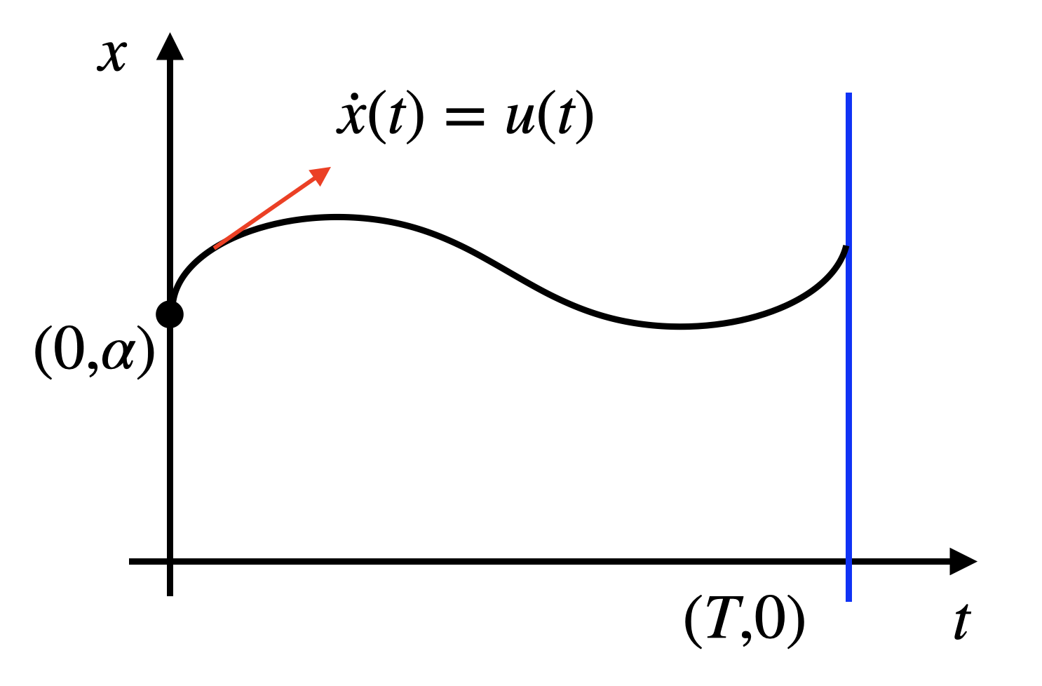
Figure 4.4: Shortest curve between a point and a line.
Let us use Pontryagin’s minimum principle to prove this. The length of any curve satisfying our condition is \[ \int_{0}^{T} \sqrt{1 + (\dot{x}(t))^2} dt, \quad x(0) = \alpha. \] To find the curve with minimum length, we can formulate an optimal control problem \[ \min_{u(t)} \int_{t=0}^T \sqrt{ 1 + u^2(t)} dt, \quad \text{subject to} \quad \dot{x}(t) = u(t), x(0) = \alpha. \]
To apply Pontryagin’s minimum principle, we first formulate the Hamiltonian \[ H(x,u,p) = g(x,u) + p^T f(x,u) = \sqrt{1 + u^2} + pu. \] The adjoint equation says \[ \dot{p}(t) = - \nabla_x H(x^\star(t),u^\star(t),p), \] which simplifies, for our problem, to \[ \dot{p}(t) = 0. \] The boundary condition of the adjoint equation is \[ p(T) = \nabla h(x^\star(T)) = 0. \] We conclude that \[ p(t) = 0, \forall t \in [0,T]. \] The optimal controller thus becomes \[ u^\star(t) = \arg\min_u H(x^\star(t),u,p(t)) = \arg\min_u \sqrt{1 + u^2} = 0, \quad \forall t \in [0,T]. \] Therefore, we have \(\dot{x}^\star(t) = u^\star(t) = 0\) for all \(t \in [0,T]\), and \(x^\star(t) = \alpha\) for all time, which is a straight line.
4.4.1 Numerical Solution of the TPBVP
When the optimal control can be solved analytically, we obtain the two-point boundary value problem (TPBVP) \[\begin{equation} \begin{cases} x^\star(0) = x_0 \\ p(T) = \nabla h(x^\star(T)) \\ \dot{x}^\star(t) = f(x^\star(t), u^\star(t)) \\ \dot{p}(t) = - \nabla_x f(x^\star(t),u^\star(t))p(t) - \nabla_x g(x^\star(t),u^\star(t)) \end{cases}, \tag{4.34} \end{equation}\] where \(u^\star(t)\) is a function of \(x^\star(t)\) and \(p(t)\). Calling \[ z(t) = \begin{bmatrix} x^\star(t) \\ p(t) \end{bmatrix}, \] we can compactly write (4.34) as \[\begin{equation} \begin{cases} b(z(0),z(T),x_0) = 0 \\ \dot{z}(t) - \phi(z(t)) = 0 \end{cases}, \tag{4.35} \end{equation}\] which has \(2n\) differential equations and \(2n\) boundary conditions and usually well defined.
4.4.1.1 Single Shooting
The idea of single shooting is straightforward: if \(p(0)\) is known in (4.34), then (i) the entire trajectory of \(z\) can be simulated forward in time, and (ii) we only need to enforce the terminal constraint of \(p(T) = \nabla h(x^\star(T))\).
Therefore, in single shooting, we denote the terminal residual \[ r_T = p(T) - \nabla h(x^\star(T)) = r_T(p_0), \] as a function of \(p(0) = p_0\) (note that evaluating this function requires simulating \(\dot{z}(t) = \phi(z(t))\)). Then we use Newton’s method to iteratively update \(p_0\) via \[ p_0^{(k+1)} = p_0^{(k)} - \eta_k \left( \frac{\partial r_T}{\partial p_0}(p_0^{(k)}) \right)^{-1} r_T(p_0^{(k)}), \] where \(\eta_k\) is a chosen step size.
In some cases, the forward simulation of the combined ODE might be an ill-conditioned problem so that single shooting cannot be employed. Even if the forward simulation problem is well-defined, the region of attraction of the Newton iteration can be very small, such that a good guess for \(p_0\) is often required.
4.4.1.2 Multiple Shooting
The single shooting method also suffers from the nonlinearity and inaccuracy brought by simulating the ODE for a long time duration \(T\).
In multiple shooting, we break the time windown \([0,T]\) into \(N\) pieces such that \[ 0 = t_0 \leq \dots \leq t_k \leq t_{k+1} \leq \dots \leq t_N = T. \] We then assign values \[ z_k = z(t_k), k = 0,\dots,N, \] as the values of \(z(t)\) at those breakpoints. The values \(z_k\) should satisfy the ODE \[ z_{k+1} = \Phi(z_k), \] where \(\Phi(\cdot)\) integrates the ODE from time \(t_k\) to \(t_{k+1}\) with initial condition \(z_k\).
We can then form a system of equations on \(z=(z_0,\dots,z_N)\) as \[\begin{equation} \begin{cases} b(z_0,z_N,x_0) = 0 \\ z_{k+1} - \Phi(s_k) = 0 \end{cases}. \end{equation}\] Denoting the vector of residuals as \[ R(z,x_0) = \begin{bmatrix} b(z_0,z_N,x_0) \\ z_{k+1} - \Phi(s_k) \end{bmatrix}, \] we can use Newton’s method to iteratively solve \(z\): \[\begin{equation} z^{(k+1)} = z^{(k)} - \eta_k \left( \frac{\partial R}{\partial z}(z^{(k)}) \right)^{-1} R(z^{(k)}). \end{equation}\]
4.5 Infinite-Horizon Problems
4.5.1 Infinite-Horizon LQR
Consider a linear time-invariant system
\[
\dot{x} = Ax + Bu,
\]
and the infinite-horizon optimal control problem
\[
\min \int_{t=0}^{\infty} (x(t)^T Q x(t) + u(t)^T R u(t)) dt, \quad x(0) = x_0.
\]
with \(Q \succeq 0, R \succ 0\).
The optimal controller takes the following linear feedback form
\[
u = - R^{-1}B^T S x,
\]
with \(S\) the solution to the continuous-time algebraic Riccati equation
\[
0 = SA + A^T S - SBR^{-1} B^T S + Q.
\]
In Matlab, given \(A,B,Q,R\), you can use lqr to compute \(K\) and \(S\).