Chapter 9 Problem Sets
Exercise 9.1 (Inscribed Polygon of Maximal Perimeter) In this exercise, we will use dynamic programming to solve a geometry problem, i.e., to find the \(N\)-side polygon inscribed inside a circle with maximum perimeter. We will walk you through the key steps of formulating and solving the problem, while leaving a few mathematical details for you to fill in.
Given a circle with radius \(1\), we can randomly choose \(N\) distinct points on the circle to form a polygon with \(N\) vertices and sides, as shown in Fig. 9.1 with \(N=3,4,5\).
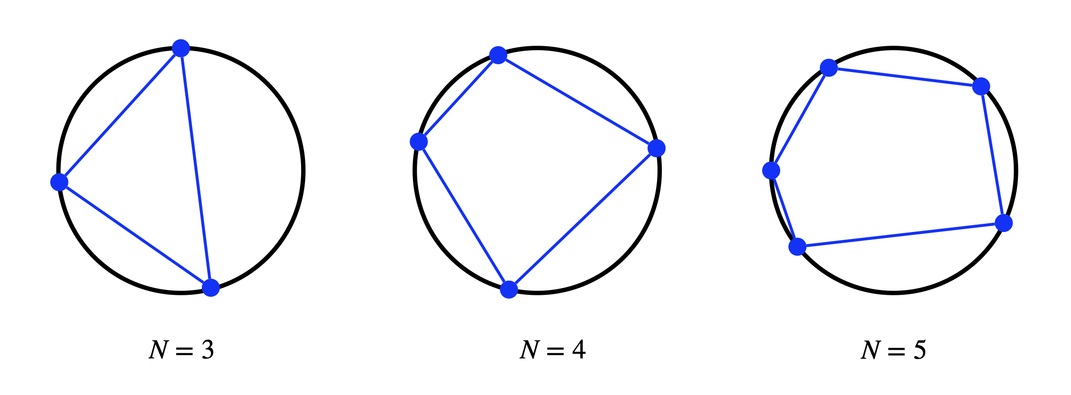
Figure 9.1: Polygons inscribed inside a circle
Once the \(N\) points are chosen, the \(N\)-polygon will have a perimeter, i.e., the sum of the lengths of its edges.
What is the configuration of the \(N\) points such that the resulting \(N\)-polygon has the maximum perimeter? I claim that the answer is when the \(N\)-polygon has edges of equal lengths, or in other words, when the \(N\) points are placed on the circle evenly.
Let us use dynamic programming to prove the claim.
To use dynamic programming, we need to definie a dynamical system and an objective function.
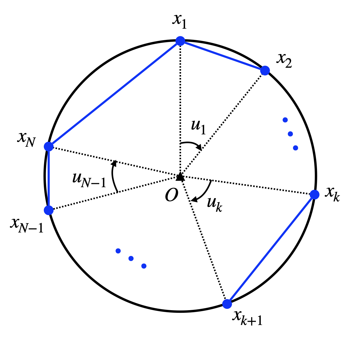
Figure 9.2: Sequential placement of N points on the circle.
Dynamical system. We will use \(\{x_1,\dots,x_N \}\) to denote the angular positions of the \(N\) points to be placed on the circle (with slight abuse of notation, we will call each of those points \(x_k\) as well). In particular, as shown in Fig. 9.2, let us use \(x_k\) to denote the angle between the line \(O-x_k\) and the vertical line (\(O\) is the center of the circle), with zero angle starting at \(12\) O’clock and clockwise being positive. Without loss of generality, we assume \(x_1 = 0\). (if \(x_1\) is nonzero, we can always rotate the entire circle so that \(x_1 = 0\)).
After the \(k\)-th point is placed, we can “control” where the next point \(x_{k+1}\) will be, by deciding the incremental angle between \(x_{k+1}\) and \(x_k\), denoted as \(u_k > 0\) in Fig. 9.2. This is simply saying the dynamics is \[ x_{k+1} = x_k + u_k, \quad k=1,\dots,N-1, \quad x_1 = 0. \]
Cost-to-go. The perimeter of the \(N\)-polygon is therefore \[ g_N(x_N) + \sum_{k=1}^{N-1} g_k(x_k, u_k), \] with the terminal cost \[ g_N(x_N) = 2 \sin \left( \frac{2\pi - x_N}{2} \right) \] the distance between \(x_N\) and \(x_1\) (see Fig. 9.2), and the running cost \[ g_k(x_k,u_k) = 2 \sin \left( \frac{u_k}{2} \right) \] the distance between \(x_{k+1}\) and \(x_k\).
Dynamic programming. We are now ready to invoke dynamic programming.
We start by setting \[ J_N(x_N) = g_N(x_N) = 2 \sin \left( \frac{2\pi - x_N}{2} \right). \] We then compute \(J_{N-1}(x_{N-1})\) as \[\begin{equation} J_{N-1}(x_{N-1}) = \max_{0< u_{N-1} < 2\pi - x_{N-1}} \left\{ \underbrace{ 2 \sin \left( \frac{u_{N-1}}{2} \right) + J_N(x_{N-1} + u_{N-1}) }_{Q_{N-1}(x_{N-1}, u_{N-1})} \right\}, \tag{9.1} \end{equation}\] where \(u_{N-1} < 2\pi - x_{N-1}\) because we do not want \(x_N\) to cross \(2\pi\).
Show that \[ Q_{N-1}(x_{N-1},u_{N-1}) = 2 \sin \left( \frac{u_{N-1}}{2} \right) + 2 \sin \left( \frac{2\pi - x_{N-1} - u_{N-1} }{2} \right), \] and \[ \frac{\partial Q_{N-1}(x_{N-1},u_{N-1})}{\partial u_{N-1}} = \cos \left( \frac{u_{N-1}}{2} \right) - \cos \left( \frac{2\pi - x_{N-1} - u_{N-1} }{2} \right). \]
Show that \(Q_{N-1}(x_{N-1},u_{N-1})\) is concave (i.e., \(-Q_{N-1}(x_{N-1},u_{N-1})\) is convex) in \(u_{N-1}\) for every \(x_{N-1} \in (0, \pi)\) and \(u_{N-1} \in (0, 2\pi - x_{N-1})\). (Hint: compute the second derivative of \(Q_{N-1}(x_{N-1},u_{N-1})\) with respect to \(u_{N-1}\) and use Proposition B.2).
With a and b, show that the optimal \(u_{N-1}\) that solves (9.1) is \[ u_{N-1}^\star = \frac{2\pi - x_{N-1}}{2}, \] and therefore \[ J_{N-1}(x_{N-1}) = 4 \sin \left( \frac{2\pi - x_{N-1}}{4} \right). \] (Hint: the point at which a concave function’s gradient vanishes must be the unique maximizer of that function)
Now use induction to show that the \(k\)-th step dynamic programming \[ J_k(x_k) = \max_{0< u_k < 2\pi - x_k} \left\{ 2 \sin\left( \frac{u_k}{2} \right) + J_{k+1}(x_k + u_k) \right\} \] admits an optimal control \[ u_k^\star = \frac{2\pi - x_k}{N-k+1}, \] and optimal cost-to-go \[ J_k(x_k) = 2(N-k+1)\sin\left( \frac{2\pi - x_k}{2(N-k+1)} \right). \]
Starting from \(x_1 = 0\), what is the optimal sequence of controls?
Hopefully now you see why my original claim is true!
(Bonus) We are not yet done for this exercise. Since you have probably already spent quite some time on this exercise, I will leave the rest of the exercise a bonus. In case you found this simple geometric problem interesting, you should keep reading as we will use numerical techniques to prove the same claim.
In Fig. 9.2, by denoting \[ u_N = 2\pi - x_N = 2\pi - (u_1 + \dots + u_{N-1}) \] as the angle between the line \(O-x_{N}\) and the line \(O-x_1\), it is not hard to observe that the perimeter of the \(N\)-polygon is \[ \sum_{k=1}^N 2 \sin \left( \frac{u_k}{2} \right). \] Consequently, to maximize the perimeter, we can formulate the following optimization \[\begin{equation} \begin{split} \max_{u_1,\dots,u_N} &\quad \sum_{k=1}^N 2 \sin \left( \frac{u_k}{2} \right) \\ \text{subject to} &\quad u_k > 0, k=1,\dots,N \\ &\quad u_1 + \dots + u_N = 2 \pi \end{split} \tag{9.2} \end{equation}\] where \(u_k\) can be seen as the angle spanned by the line \(x_k - x_{k+1}\) with respect to the center \(O\) so that they are positive and sum up to \(2\pi\).
- Show that the optimization (9.2) is convex. (Hint: first show the feasible set is convex, and then show the objective function is concave over the feasible set.)
Now that we have shown (9.2) is a convex optimization problem, we know that pretty much any numerical algorithm will guarantee convergence to the globally optimal solution.
It is too much to ask you to implement a numerical algorithm on your own, as that can be a one-semester graduate-level course (Nocedal and Wright 1999). However, Matlab provides a nice interface, fmincon, to many such numerical algorithms, and let me show you how to use fmincon to solve (9.2) so we can numerically prove our claim.
- I have provided most of the code necessary for solving (9.2) below. Please fill in the definition of the function
perimeter(u), and then run the code in Matlab. Show your results for \(N=3,10,100\). Do the solutions obtained fromfminconverify our claim?
clc; clear; close all;
% number of points to be placed
N = 10;
% define the objective function
% fmincon assumes minimization
% We minimize the negative perimeter so as to maximize the perimeter
objective = @(u) -1*perimeter(u);
% choose which algorithm to use for solving
options = optimoptions('fmincon', 'Algorithm', 'interior-point');
% supply an initial guess
% since this is a convex problem, we can use any initial guess
u0 = rand(N,1);
% solve
uopt = fmincon(objective,u0,... % objective and initial guess
    -eye(N),zeros(N,1),... % linear inequality constraints
    ones(1,N),2*pi,... % linear equality constraints
    [],[],[],... % we do not have lower/upper bounds and nonlinear constraints
    options);

% plot the solution
x = zeros(N,1);
for k = 2:N
    x(k) = x(k-1) + uopt(k-1);
end
figure;
% plot a circle
viscircles([0,0],1);
hold on
% scatter the placed points
scatter(cos(x),sin(x),'blue','filled');
axis equal;

%% helper functions
% The objective function
function f = perimeter(u)
% TODO: define the perimeter function here.
end
Exercise 9.2 (LQR with Constraints) In class we worked on the LQR problem where the states and controls are unbounded. This is rarely the case in real life – you only have a limited amount of control power, and you want your states to be bounded (e.g., not entering some dangerous zones).
For linear systems with convex constraints on the control and states, the seminal paper (Bemporad et al. 2002) investigates the landscape of the optimal cost-to-go and controller.
In this exercise, let us use convex optimization to numerically study a toy problem.
Consider a variant of the LQR problem (2.2) where the controls are bounded between \([-u_{\max}, u_{\max}]\), the system matrices \(A_k, B_k\) are constant, and the dynamics is deterministic: \[\begin{equation} \begin{split} J(x_0) = \min_{u_{0},\dots,u_{N-1} \in [-u_{\max},u_{\max}]} &\quad x_N^T Q_N x_N + \sum_{k=0}^{N-1} (x_k^T Q_k x_k + u_k^T R_k u_k) \\ \text{subject to} &\quad x_{k+1} = A x_k + B u_k, k=0,\dots,N-1 \end{split} \tag{9.3} \end{equation}\] We assume \(Q_k\succeq 0\) for \(k=0,\dots,N\) and \(R_k \succ 0\) for all \(k=0,\dots,N-1\).
Show that Problem (9.3), when \(x_0\) is given, is a convex optimization problem.
Discretize the continuous-time double integrator dynamics \[ \ddot{q} = u, \quad u \in [-1,1] \] in the form of \(x_{k+1} = A x_k + B u_k\) with a constant \(dt\) time discretization. (Hint: take \(x = [q,\dot{q}]\) as the state vector.)
Fix \(N=50\), \(dt=0.1\) and choose your favorite \(Q_k\) and \(R_k\). Solve the convex optimization (9.3) at a dense grid of \(x_0\) (e.g., using CVX or cvxpy). Plot the optimal cost-to-go \(J(x_0)\), and the optimal controls \(u_0(x_0),\dots,u_{N-1}(x_0)\). For the optimal controls, you can just plot one of the controls such as \(u_0(x_0)\). You may want to use the Matlab function
surf. (Hint: you will most likely benefit from Appendix B.2.)Increase \(N\) and decrease \(dt\), repeat (c). Do you get more fine-grained plots of the optimal cost-to-go and controls? (When you increase \(N\), the convex optimization has more variables to optimize, so there is a limit at which the solver takes too much time.)
(Bonus) We only have constraints on the control so far. What if you add constraints to the states as well? For example, you can try limiting the velocity \(\dot{q}\) to be at least \(0.1\) by adding \(\dot{q}_k \geq 0.1\) for some k. How will \(J\) and \(u\) change?
(Bonus) Can you write down the KKT optimality conditions of (9.3) and explain what you have observed from the numerical experiments? (Hint: KKT optimality conditions can be found in Theorem B.2.)
Exercise 9.3 (Cart Pole System) In this exercse, let us study the cart-pole system (we saw the video of human-controlled version in our first lecture), another interesting nonlinear control problem, and reinforce our knowledge about LQR.
Our task is to balance a pendulum on a cart by horizontally moving the cart. Fig. 9.3 gives an illustration of the system. See this video for an actual robotic implementation.
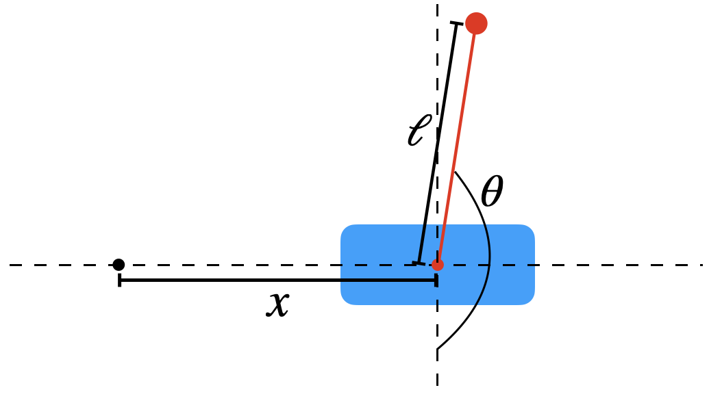
Figure 9.3: Illustration of cart-pole problem
With the above illustration, we parameterize the system with two scalars: \(x\) represents the current location of the cart, while \(\theta\) is the angle between current pole and the stable equilibrium. Therefore, our goal is to study the motion of the cart-pole system with a horizonal control \(f\). We assume hereafter the system is ideal such that there is no friction, and the mass of the pole concentrates at the free end point.
- (Bonus) For those of you who have background in rigid-body dynamics, this is an opportunity for you to apply your knowledge. However, feel free to skip this subproblem and it won’t affect the rest of the exercise. Denote the mass of cart and pole as \(m_c\) and \(m_p\), respectively. Derive the equations of motion: \[\begin{equation} \left(m_c+m_p\right) \ddot{x}+m_p l \ddot{\theta} \cos \theta-m_p l \dot{\theta}^2 \sin \theta=f, \tag{9.4} \end{equation}\] \[\begin{equation} m_p l \ddot{x} \cos \theta+m_p l^2 \ddot{\theta}+m_p g l \sin \theta=0. \tag{9.5} \end{equation}\] (Hints: compute the Lagrangian of the system and the corresponding Lagrangian equations. Analyzing the two objects separately also works.)
Translate the equations in (a) into the basic state-space dynamics form \[\begin{equation} \dot{\mathbf{x}}=F(\mathbf{x}, \mathbf{u}). \tag{9.6} \end{equation}\] What are \(\mathbf{x},\mathbf{u},F\) here? (Hint: try \(\mathbf{x}=[x,\theta,\dot{x},\dot{\theta}]^\top\).)
Linearize the dynamics in (b) around the unstable equilibrium where \(\theta^*=\pi\) and \(x^*=\dot{x}^*=\dot{\theta}^*=0.\) (i.e., the pole is in the upright position and the cart stay at zero.) The result should be in the form of \[\begin{equation} \dot{\Delta\mathbf{x}}=A\Delta\mathbf{x}+B\Delta\mathbf{u}, \tag{9.7} \end{equation}\] where \(\Delta\mathbf{x} = \mathbf{x}-\mathbf{x}^*\) and \(\Delta\mathbf{u}=\mathbf{u}-\mathbf{u}^*\).
Define the linearization error \(e(\mathbf{x}, \mathbf{u}):=\|F(\mathbf{x}, \mathbf{u}) - (A\Delta\mathbf{x}+B\Delta\mathbf{u})\|^2\). Simulate the original system (9.6) and the linearized system (9.7) with the same initial condition. How does the linearization error change over time? Provide at least three different initialization results.
(Hints: (i) Sanity check: intuitively the error should not depend on the initial location \(x\), and it should have symmetry. Is that true in your simulation?
(ii) In the same unstable position, how does push/pull (positive/negative) force change the results?)Convert the continuous-time dynamics in (9.7) to discrete-time with a fixed time-discretization. Then design an LQR controller to stabilize the cart-pole at the unstable equilibrium. Does the LQR controller succeed for all initial conditions you tested? (Hint: try several initial conditions where the end point of the pole is above or below the horizontal line.) You may want to take a look at the LQR example for the simple pendulum in Example 2.1.
Exercise 9.4 (Trajectory Optimization) Let us use this exercise to practice your skills in implementing trajectory optimization.
Consider a dynamical system \[ x = \begin{bmatrix} x_1 \\ x_2 \end{bmatrix}, \quad \dot{x} = f(x,u) = \begin{bmatrix} (1-x_2^2)x_1 - x_2 + u \\ x_1 \end{bmatrix}, \quad x(0) = x_0 = \begin{bmatrix} 0 \\ 1 \end{bmatrix}. \]
With \(T=10\), consider the following optimal control problem \[\begin{equation} \begin{split} \min_{u(t),t \in [0,T]} & \quad \int_{t=0}^T \Vert x(t) \Vert^2 + u(t)^2 dt \\ \text{subject to} & \quad \dot{x} = f(x,u), \quad x(0) = x_0 \\ & \quad u(t) \in [-1,1],\forall t \in [0,T]. \end{split} \end{equation}\]
Solve the problem using direct multiple shooting with \(N=50\) time intervals.
Solve the problem using direct collocation with \(N=50\).
Plot the optimized control signal and resulting state trajectory for both a and b. You probably want to refer to the source codes of Example 3.6 and 3.7.
Exercise 9.5 (Policy Iteration of Shortest Path) In Example 2.2, we used value iteration to solve the shortest path problem with obstacles. In this exercise, we will implement policy iteration. Instead of value iteration that updates the Q-function by \(Q^{(k+1)} = \mathcal{T}Q^{(k)}\) where \(\mathcal{T}\) is the Bellman optimality operator defined in (2.27), we use a different update rule:
Initialize the policy \(\pi_0\).
For \(k=0,1,2,\ldots\), compute \(Q_{\pi_k}\) via (2.24). Then update policy by greedy method \(\pi_{k+1}=\pi_{Q^{\pi_k}}\) (see (2.26) for the definition of \(\pi_Q\)).
Now try to solve the following problems.
With the same obstacles in Fig. 2.3, implement the above policy iteration algorithm. Can you recover the cost-to-go and shortest path found in the example?
We designed the cost function \(g\) to be \(20\) when there is an obstacle. Is there a lower bound on this value, such that the shortest path with any starting point will still avoid obstacles? If yes, how will the lower bound change with different obstacle structures? (Bonus) With the assumption that the grids are connected, give a conjecture on the maximum of the lower bound.
If it is allowed to go diagonally (for example, from (4,4) to (3,5)), how will the results change?
(Bonus) Beyond iterative algorithms, there is another formulation of the problem in linear programming. Try to implement the following problem: \[\max_{J} \sum_{x}J(x),\quad s.t. J(x)\le g(x,u) + \gamma\sum_{x'}P(x'|x,u)J(x'),\ \forall x,u.\] What can you find? (Hint: formulate the problem as a linear programming problem.)
Exercise 9.6 (Verifying Control Lyapunov Function for the Double Integrator) Consider the following discrete-time double integrator dynamics \[ x_{t+1} = \underbrace{\begin{bmatrix} 1 & 1 \\ 0 & 1 \end{bmatrix}}_{A} x_t + \underbrace{\begin{bmatrix} 0 \\ 1 \end{bmatrix}}_{B} u_t, \] with control constraints \[ u \in \mathcal{U} = [-1, 1]. \] We do not enforce any state constraint on \(x\), that is \(\mathcal{X} = \mathbb{R}^2\).
Receding horizon controller. We aim to regulate the system at the origin, and design the following receding horizon controller (RHC) with horizon \(N=3\) \[\begin{equation} \begin{split} \min_{u(0),\dots,u(N-1)} & \quad x(N)^T P x(N) + \sum_{k=0}^{N-1} x(k)^T Q x(k) + u(k)^T R u(k) \\ \text{subject to} & \quad u(k) \in \mathcal{U}, \forall k=0,\dots,N-1 \\ & \quad x(k+1) = A x(k) + B u(k), \forall k = 0,\dots,N-1 \\ & \quad x(0) = x_t, \end{split} \tag{9.8} \end{equation}\] where \(x_t\) is the system state at time \(t\), and \(P,Q,R\) matrices are designed as follows \[ Q = \begin{bmatrix} 1 & 0 \\ 0 & 0 \end{bmatrix}, \quad R = 1, \quad P = \begin{bmatrix} 0.1 & 0 \\ 0 & 0.1 \end{bmatrix}. \]
Implement the RHC in (9.8), and run the RHC with initial system state \(x_0 = [2;1]\). Plot the system trajectory on a 2D plane like Fig. 3.24.
From Theorem 3.3, we know that a sufficient condition for the stability of RHC is that the terminal cost, in our example is \(p(x) = x^T P x\), needs to satisfy (3.40). When \(p(x)\) satisfies (3.40), we say \(p(x)\) is a control Lyapunov function (CLF). Instantiating (3.40) for this exercise, it becomes (recall that we do not have terminal constraint, i.e., \(\mathcal{X}_f = \mathbb{R}^2\)): \[\begin{equation} \rho = \min_{u \in \mathcal{U}} \ \ (Ax + Bu)^T P (Ax + Bu) - x^T P x + x^T Q x + u^T R u \leq 0, \quad \forall x \in \mathbb{R}^2. \tag{9.9} \end{equation}\] Computing \(\rho\) for all \(x\) in \(\mathbb{R}^2\) is difficult, so I will ask you to compute \(\rho\) along the state trajectory generated by RHC in (a). Compute and plot the trajectory of \(\rho\).
From Proposition 2.2, we know the optimal cost-to-go of the unconstrained infinite-horizon LQR problem with \(x(0) = x\) \[ J_{\infty}(x) = \min_{u(0),\dots} \ \ \sum_{k=0}^{\infty} u(k)^T R u(k) + x(k)^T Q x(k), \quad \text{subject to} \quad x(k+1) = A x(k) + B u(k), \] is a quadratic function \[ J_{\infty}(x) = x^T S x, \] where \(S\) can be computed by solving the algebraic Riccati equation. Now use Matlab or Python to compute \(S\) (e.g., using
dlqrin Matlab) for the double integrator.Redo (a) and (b) by using \(S\) in (c) as the terminal cost, i.e., setting \(P=S\). Plot the state trajectory, as well as the trajectory of \(\rho\).
Redo (a) and (b) by using \(0.1S\) and \(10S\) as the terminal cost, i.e., setting \(P=0.1S\) and \(P=10S\). Plot the state trajectory, as well as the trajectory of \(\rho\).
Exercise 9.7 (Polyhedral Controllable and Reachable Sets) In this exercise, we aim to compute controllable and reachable sets explicitly, rather than implementing MPT.
A bounded polyhedron in \(\mathbb{R}^n\) can be expressed as the convex hull of a finite set of points (vertices) \(V = \{V_1, \ldots, V_k\}\subset \mathbb{R}^n\). Show that a linear transform of such a polyhedron is simply tranforming its vertices, namely, \[A\text{conv}(V)+b = \text{conv}(AV)+b,\] where \(A\in\mathbb{R}^{m\times n},\ b\in\mathbb{R}^m\).
The exact definition of a (closed) polyhedron \(\mathcal{P}\) is a set defined by finite number of linear inequalities \(\mathcal{P} = \{x\in\mathbb{R}^n\mid Hx\le h \}\) where \(H\in\mathbb{R}^{m\times n},\ h\in\mathbb{R}^m\). Let \(A\in\mathbb{R}^{n\times n}\) be an invertible matrix, \(b\in\mathbb{R}^n\). Suppose the linear transformed polyhedron \(A\mathcal{P}+b\) has representation \[\{y\in\mathbb{R}^n\mid H^\prime y\le h^\prime \}.\] What are \(H^\prime\) and \(h^\prime\)?
With the same setting as Example 3.10, consider linear system \[ x_{t+1} = \begin{bmatrix} 1.5 & 0 \\ 1 & -1.5 \end{bmatrix} x_t + \begin{bmatrix} 1 \\ 0 \end{bmatrix} u_t \] with state and control constraints \[ \mathcal{X} = [-10,10]^2, \quad \mathcal{U} = [-5,5]. \] Compute \(\text{Pre}(\mathcal{X})\) and \(\text{Suc}(\mathcal{X})\) in the form of \(\{x\in\mathbb{R}^n\mid Hx\le h \}\). What are the vertices of two sets respectively?
(Hints: Denote the dynamics as \(x_{t+1} = Ax_t+Bu_t\). For the successor set, \[\text{Suc}(\mathcal{X}) = \cup_{u\in\mathcal{U}}\{x:\exists x'\in\mathcal{X},\text{ s.t., }Ax'+Bu = x\} = \cup_{u\in\mathcal{U}}(A\mathcal{X} + Bu).\] What is \(A\mathcal{X} + Bu\) for each \(u\)? Will the shape of \(A\mathcal{X} + Bu\) change when changing \(u\)? The conclusion in (b) might help.
Similarly, for the precursor set, \[\text{Pre}(\mathcal{X}) = \cup_{u\in\mathcal{U}}\{x:Ax+Bu \in \mathcal{X}\} = \cup_{u\in\mathcal{U}}A^{-1}(\mathcal{X} - Bu).\] Mimic the computation of the successor set.)Continued with the results in (c), compute one-step controllable set \(\mathcal{K}_1(\mathcal{X}) = \text{Pre}(\mathcal{X}) \cap \mathcal{X}\).
(Hints: There are 4 inequalities for each of the two sets. Any redundancy in those 8 inequalities when combining them together?)From the above questions, we get the intuition of how the MPT compute controllable set:
- Obtain the representation of precursor set;
- Intersect the precursor set with the feasible domain \(\mathcal{X}\);
- Remove redundant (useless) inequalities.
Provided the following algorithm that removes redundancy of a polyhedral representation, write the codes to find \(\mathcal{K}_1(\mathcal{X})\) without using MPT. Does the outcome match your results in (d)?
Algorithm: Find redundacy-free representation of a polyhedron
Input: \(H\in\mathbb{R}^{m\times n}\) and \(h\in\mathbb{R}^m\) that represents \(\mathcal{P} = \{x\in\mathbb{R}^n\mid Hx\le h \}\)
Output: \(H_0\in\mathbb{R}^{m_0\times n}\) and \(h_0\in\mathbb{R}^{m_0}\) that represents \(\mathcal{P}\) without redundancy
\(\mathcal{I} \leftarrow \{1,\ldots, m\}\)
For \(i=1\) to \(m\)
\(\mathcal{I}\leftarrow \mathcal{I}\setminus\{i\}\)
\(f^*\leftarrow\max_x H_i x,\ s.t. H_{\mathcal{I}}x\le h_{\mathcal{I}}, H_i x\le h_i + 1\)
%% \(H_i\) is the \(i\)-th row of \(H\), \(H_{\mathcal{I}}\) concatenates rows of \(H\) with index in \(\mathcal{I}\)
If \(f^* > h_i\) Then \(\mathcal{I}\leftarrow \mathcal{I}\cup \{i\}\)
\(H_0\leftarrow H_{\mathcal{I}}, h_0\rightarrow h_{\mathcal{I}}\)
Exercise 9.8 (Certified Region of Attraction of Clipped LQR Controller) In this exercise, let us use the simple pendulum as an example to (i) recognize the difficulty of nonlinear control in the presence of control limits, and (ii) appreciate the power of Lyapunov analysis and Sums-of-Squares (SOS) programming.
A starting script for this exercise can be found here, where you need to fill out some specific details to finish this exercise.
Let us consider the continuous-time pendulum dynamics \[\begin{equation} \dot{x} = \begin{bmatrix} x_2 \\ \frac{1}{ml^2} (u - b x_2 + mgl \sin x_1) \end{bmatrix} \tag{9.10} \end{equation}\] where \(x_1\) is the angular position of the pendulum, and \(x_2\) is the angular velocity. Note that the dynamics above is written such that \(x=0\) represents the upright position.
In the case of no control saturation, i.e., \(u \in \mathbb{R}\), stabilizing the pendulum at \(x=0\) is easy, we can linearize the dynamics at \(x=0\) and obtain
\[
\dot{x} \approx \underbrace{\begin{bmatrix} 0 & 1 \\ \frac{g}{l} & - \frac{b}{ml^2} \end{bmatrix}}_{A} x + \underbrace{\begin{bmatrix} 0 \\ \frac{1}{ml^2} \end{bmatrix}}_{B} u.
\]
We then solve an infinite-horizon LQR problem
\[
\min \int_{t=0}^{\infty} x(t)^T Q x(t) + u(t)^T R u(t) dt, \quad \text{subject to} \quad x(0) = x_0.
\]
The solution to this LQR problem can be written in closed form, see Section 4.5.1.
Calling the Matlab lqr function (which is for continuous-time LQR), we can get a feedback controller
\[\begin{equation}
u(x) = - Kx,
\tag{9.11}
\end{equation}\]
with the optimal cost-to-go
\[\begin{equation}
J(x_0) = x_0^T S x_0,
\tag{9.12}
\end{equation}\]
with \(K\) and \(S\) constant matrices.
Control saturation. Assume now our control has hard bounds, i.e., \[ u \in [-u_{\max}, u_{\max}]. \] We wish to keep using the LQR controller (9.11). Therefore, our saturated controller will be \[\begin{equation} \bar{u}(x) = \text{clip}(u(x),-u_{\max},u_{\max}) = \text{clip}(-Kx,-u_{\max},u_{\max}), \tag{9.13} \end{equation}\] where the \(\text{clip}\) function is defined as \[ \text{clip}(u,-u_{\max},u_{\max}) = \begin{cases} u_{\max} & \text{if} \quad u \geq u_{\max} \\ u & \text{if} \quad -u_{\max} \leq u \leq u_{\max} \\ -u_{\max} & \text{if} \quad u \leq - u_{\max} \end{cases}. \]
A natural question is: can the saturated controller \(\bar{u}(t)\) in (9.13) still stabilize the pendulum?
Let’s simulate the pendulum and the controller to investigate this. We will use the parameter \(m=1,g=9.8,l=1,b=0.1\), and \(u_{\max} = 2\). For the LQR cost matrix, let us use \(Q = I\) and \(R = 1\).
- Compute the LQR gain \(K\) and implement the saturated controller (9.13). In a region \(\mathcal{X} = [-0.2\pi, 0.2\pi] \times [-0.2\pi, 0.2\pi]\), sample \(N=1000\) initial states, and for each initial state, simulate the system under the saturated controller using
ode45orode89. There will be some initial states from which the pendulum gets stabilized and others from which the pendulum fails to be stabilized. Plot the stabilized initial states as “circles”, and the non-stabilized initial states as “squares” on a 2D plot. (Hint: you should get something like Fig. 9.4.)
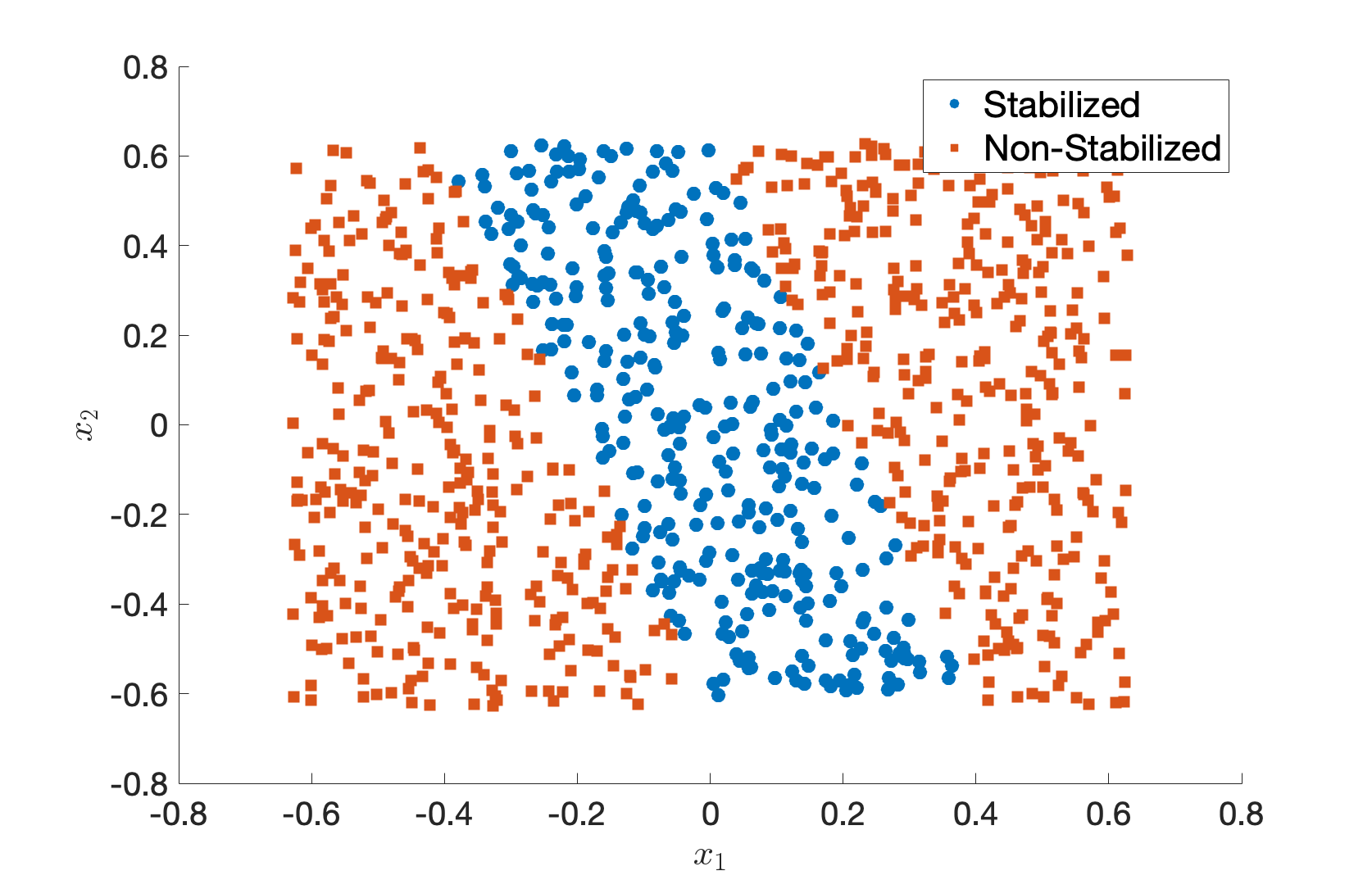
Figure 9.4: Example of stabilized and non-stabilized initial states.
The plot in Fig. 9.4 intuitively makes sense: when the initial state is very close to \(0\), the saturated controller can still stabilize the pendulum.
Now our goal is to use Sums-of-Squares and Lyapunov analysis to get a certified region of stabilization, also known as the region of attraction (ROA), under the saturated control.
Approximate polynomial dynamics. The SOS tool requires the system dynamics to be polynomial. The dynamics in (9.10) is polynomial except the term \(\sin x_1\). Therefore, we perform a Taylor expansion of \(\sin x_1\) \[ \sin x_1 = x_1 - \frac{x_1^3}{3!} + \frac{x_1^5}{5!} + \dots, \] leading to an approximate polynomial dynamics \[\begin{equation} \dot{x} = \bar{f}(x,u) = \begin{bmatrix} x_2 \\ \frac{1}{ml^2} \left(u - b x_2 + mgl \left(x_1 - \frac{x_1^3}{3!} + \frac{x_1^5}{5!} \right) \right) \end{bmatrix}. \tag{9.14} \end{equation}\]
Candidate ROA. We want to certify the following candidate ROA \[ \Omega_\rho = \{x \in \mathbb{R}^2 \mid J(x) :=x^T S x \leq \rho \} \] for some \(\rho > 0\), and \(S\) is exactly the LQR cost-to-go in (9.12). Since \(J(x)\) is already positive definite (because \(S \succ 0\)), \(\Omega_\rho\) will look like an elliptical region around the origin. To certify all initial states inside \(\Omega_\rho\) can be stabilized, we need \(\dot{J}(x)\) to be negative definite on \(\Omega\), under the saturated LQR controller (9.13) (according to Theorem 5.2), that is to say \[ \dot{J}(x) = \frac{\partial J}{\partial x} \bar{f}(x, \bar{u}(x)) < 0, \quad \forall x \in \Omega_\rho \backslash \{ 0 \}. \] A sufficient condition for the above equation to hold is \[\begin{equation} - \frac{\partial J}{\partial x} \bar{f}(x, \bar{u}(x)) - \epsilon \Vert x \Vert^2 \quad \text{ is SOS on } \Omega_\rho. \tag{9.15} \end{equation}\] for some \(\epsilon > 0\) (do you see this?).
The condition (9.15) is almost ready for us to implement in SOSTOOLS. However, there is one last issue. The saturated controller \(\bar{u}(x)\) is not a polynomial!
The last trick. Fortunately, we can use a trick here to save us. A closer look at (9.15) and the saturated controller \(\bar{u}(x)\) shows that it is equivalent to asking \[\begin{equation} \begin{split} - \frac{\partial J}{\partial x} \bar{f}(x, u_{\max}) - \epsilon \Vert x \Vert^2 \quad \text{ is SOS on } \quad \Omega_\rho \cap \{ x \mid u(x) \geq u_{\max} \} \\ - \frac{\partial J}{\partial x} \bar{f}(x, u(x)) - \epsilon \Vert x \Vert^2 \quad \text{ is SOS on } \quad \Omega_\rho \cap \{ x \mid -u_{\max} \leq u(x) \leq u_{\max} \} \\ - \frac{\partial J}{\partial x} \bar{f}(x, - u_{\max}) - \epsilon \Vert x \Vert^2 \quad \text{ is SOS on } \quad \Omega_\rho \cap \{ x \mid u(x) \leq -u_{\max} \}. \end{split} \tag{9.16} \end{equation}\] Essentially, (9.16) breaks the SOS condition into three cases, each corresponding to one case in the \(\text{clip}\) function. (1) If \(u(x) \geq u_{\max}\), then the first equation takes \(u_{\max}\) to be the controller, (2) If \(u(x) \leq -u_{\max}\), then the third equation takes \(-u_{\max}\) to be the controller, (3) otherwise, the second equation takes \(u(x)=-Kx\) to be the controller. Condition (9.16) has three SOS constraints and can be readily implemented using SOSTOOLS. We will use \(\epsilon = 0.01\).
- Choose \(\rho = 1\), and implement the SOS conditions in (9.16) with a chosen relaxation order \(\kappa\) (in the code I choose \(\kappa=4\)). Is the SOS program feasible (i.e., does the SOS program produce a certificate)? If so, plot the boundary of \(\Omega_\rho\) on top of the samples plot in Fig. 9.4. Does \(\Omega_\rho\) agree with the samples? (Hint: you should see a plot similar to Fig. 9.5.)
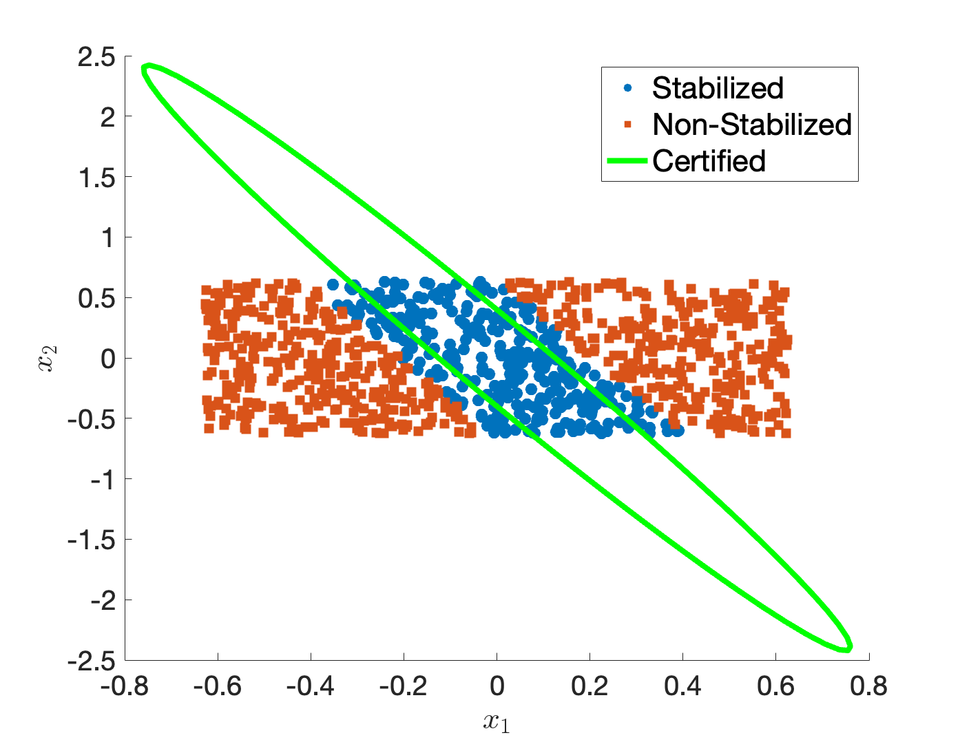
Figure 9.5: Certified Region of Attraction.
- Now try \(\rho = 2,3,4,5\), for which values of \(\rho\) the SOS program is feasible, and for which values of \(\rho\) the SOS program becomes infeasible?
Exercise 9.9 (Energy pumping of Simple Pendulum) In Exercise 9.8, we have studied the region of attraction of the Clipped LQR Controller. The conclusion we got there is, once we enter the region of attraction \(\Omega_\rho\) (the green elliptical region in Fig. 9.5), we can switch to the clipped LQR controller and it guarantees stabilization towards the upright position.
In this exercise, we are going to design a controller that can swing up the pendulum to enter the region of attraction.
The total energy of the pendulum is given by \[ E = \frac{1}{2} m l^2 x_2^2 + mgl\cos x_1,\] where \(x_1\) and \(x_2\) are notations in (9.10).
With the dynamics in (9.10), one can obtain the change of energy over time: \[ \dot E = \color{red}{h(x,u)}\cdot x_2.\] Find the expression of \(h(x,u)\).
Our desired energy is the one with the upright equilibruim: \(E^d = mgl.\) Define the energy of difference \[\tilde{E} = E - E^d.\] Find the expression of \(\dot{\tilde{E}}\).
Now consider the feedback controller of the form \[ u = -k x_2 \tilde{E} + b x_2.\] Find the expression of \(\dot{\tilde{E}}\). (Bonus) Explain heuristically why the controller works.
However, our controller has saturation as before: \[\bar{u}(x) = \text{clip}(u(x),-u_{\max},u_{\max}).\] Set the parameters the same as the previous exercise and \(k=1\). Simulate the system under the saturated controller with initial state \((x_1,x_2)=(\pi,1).\) Will the state hit the candidate ROA \(\Omega_\rho\) with \(\rho=2\)? If yes, stop the system once it hits the region, and draw the trajectory on the Figure similar to Fig. 9.5. Try \(k=0.01, 0.1,1,10\), which one hits the region the fastest?
Congrats! We have designed a full nonlinear controller (energy pumping + clipped LQR) that guarantees swing-up of the pendulum from any initial state to the upright position. Try the controller for yourself.