Chapter 7 Geometric Vision
In this Chapter, we introduce the fundamentals of geometric vision, a (classical) branch of computer vision that seeks to estimate geometric models (e.g., 3D rotations, translations, and points) from sensor measurements (e.g., images and point clouds). There are two goals for introducing geometric vision.
In the output feedback Chapter 6, we see that the full state \(x\) of a dynamical system is often not available, and needs to be estimated from the measurement signal \(y\) that satisfies \[ y(t) = h(x(t),u(t)) \] potentially plus some noise. In Chapter 6, we studied the case where \(y\) is part of the state \(x\), often the position \(q\) of a second-order system \(x=[q;\dot{q}]\). For example, in the pendulm swing-up example, we assume the angular position \(\theta\) is observed, but not the angular velocity \(\dot{\theta}\). However, in many practical applications, the measurement signal \(y\) does not directly tell us the position \(q\), and we need to estimate \(q\) from \(y\). For instance, a quadcopter needs to estimate its position from its onboard cameras. Once we obtain an estimated \(q\) from \(y\), we can use the observer synthesis methods in Chapter 6 to obtain the full state estimation.
The estimation community and the control community are a bit separated (at least in my opinion), despite that they share a lot of common tools, especially optimization. We will see that estimating \(q\) from \(y\), where \(y\) could be a high-dimensional image, is often formulated as an optimization problem that is difficult to solve. However, using the SOS tool we developed in Chapter 5, we can actually solve the optimization problem to global optimality.
7.1 3D Rotations and Poses
7.1.1 Rotation matrices
The first part is a quick recap of the basics in linear algebra.
Definition 7.1 (Orthogonal Matrix) We call a \(n\times n\) square matrix \(A\) orthogonal if the column of \(A\) is orthogonal to each other and all the column vectors have unit length. The set of all \(n\times n\) orthogonal matrices is denoted as \(O(n)\).
Below are some basic properties of orthogonal matrices:
Proposition 7.1 (Property of Orthogonal Matrix) Let \(A\) be a \(n\times n\) orthogonal matrix. Then:
\(A^T = A^{-1}\) and \(A^T\) is also a orthogonal matrix.
For every orthogonal matrices \(A,B\), \(AB\) is also a orthogonal matrix.
\(\det(A) = \pm 1\).
\(A\) preserves dot product, i.e. \(<x,y> = <Ax,Ay>\), thus preserves the length of a vector, i.e. \(\|Ax\|_2 = \|x\|_2\).
All the eigenvalues of \(A\) have modulus one.
Proof. We only offer the proof of the last property. Consider any eigenvalue \(\lambda\) of \(A\), and \(x\) be its eigenvector. We have \(<x,x> = <A^TAx,x>=<Ax,Ax> = |\lambda|^2<x,x>\), thus \(|\lambda|=1\).
There are two types of orthogonal matrices, categorized by determinant \(1\) and \(-1\). Those with determinant \(1\) are called rotation matrices. The set of rotation matrices is denoted as \(SO(n)\) (Special Orthogonal). In the world of robotics and most engineering fields, we care about \(SO(3)\) the most. Below are some basic properties of \(3\times 3\) rotation matrices:
Proposition 7.2 (Property of Rotation Matrix) Let \(A\) be a \(3\times 3\) orthogonal matrix. Then:
\(\det(A) = \pm 1\)
For every rotation matrices \(A,B\), \(A^T\),\(AB\) are also rotation matrices.
\(A\) always has an eigenvalue \(1\). If \(A\) is not identity, \(A\) either has two conjugate complex eigenvalues not equal to 1, or has two eigenvalues -1.
Proof. We can only prove the last property.
From the property of orthogonal matrix, we know that all eigenvalues have modulus one. First, note that there must exist at least one real eigenvalue. Because eigenvalues with nonzero imaginary parts always come in pair and 3 is an odd number.
Then there are two possible cases: (1) All the eigenvalues are real; (2) There is only one eigenvalue.
For case one, note that the determinant of a matrix is the product of all eigenvalues, then rotation matrix can’t have all the eigenvalues -1.
For case two. The product of the pairing complex eigenvalues is the square of the modulus of the eigenvalue, which is 1. So the real eigenlvalue left must be 1.
Finally if all the eigenvalues of \(A\) are 1, then \(A\) must be identity.
7.1.2 Coordinate Frame
Coordinate frames are a set of orthogonal basis (containing three axes) attached to a certain body at a point. It serves as the tool to describe the position of points relative to that body. Conventionally, coordinate frames are right-handed. We will encounter different frames in applications, including: (1) Robot (robot frame “\(r\)”), (2) Sensor on the robot (e.g. camera frame ‘\(c\)’), (3) A fixed location in the world (world frame “\(w\)”)
It’s worth metion that, denote \(\vec{x},\vec{y},\vec{z}\) as the three axes of the coordinate frame, then the right-handed property can be expressed as: \(\vec{x}\cdot(\vec{y}\times \vec{z}) = 1\), which is the same as \(\det ([\vec{x},\vec{y},\vec{z}]) = 1\). So the matrix \([\vec{x},\vec{y},\vec{z}]\) is a rotation matrix.
It’s natural for us to ask three questions: (1) How to express a point in a given frame? (2) How to represent a frame \(r\) with respect to a frame \(w\)? (3) How to translate the coordinate of a point in different frames?
(1) How to express a point in a given frame?
Let’s consider a reference frame \(r\) and denote the the three axes attached to it as \(\vec{x^r},\vec{y^r},\vec{z^r}\). Then for any point \(p\), we care about the vector pointing from the origin of the frame to \(p\). We slightly abuse the notation and let that vector called \(p\).(Since we will only care about the vector) Then, we can express \(p\) as the combination of the basis, i.e. \[p = p^r_x \vec{x^r}+p^r_y\vec{y^r}+p^r_z\vec{z^r} = \begin{bmatrix} \vec{x^r},\vec{y^r},\vec{z^r}\end{bmatrix} \begin{bmatrix} p^r_x\\p^r_y\\p^r_z \end{bmatrix}\] Thus we can fully describe point \(p\) with three scalars \(p^r_x,p^r_y,p^r_z\), which is called the coordinates of \(p\) with respect to the frame \(r\).
(2) How to represent a frame \(r\) with respect to a frame \(w\)?
Now we consider how to describe frame \(w\) in frame \(r\). Let’s focus on the simple case where the origin of the two coordinate systems coincide. Then we can express the axes \(\vec{x^w},\vec{y^w},\vec{z^w}\) in frame \(r\) directly. For example, thanks to the orthogonality, we can get:\[\vec{x^w} = <\vec{x^w},\vec{x^r}>\vec{x^r} +<\vec{x^w},\vec{y^r}>\vec{y^r} + <\vec{x^w},\vec{z^r}>\vec{z^r} = \begin{bmatrix} \vec{x^r},\vec{y^r},\vec{z^r}\end{bmatrix}\begin{bmatrix} <\vec{x^w},\vec{x^r}>\\ <\vec{x^w},\vec{y^r}>\\<\vec{x^w},\vec{z^r}> \end{bmatrix}\] So we can get: \[\begin{bmatrix} \vec{x^w},\vec{y^w},\vec{z^w} \end{bmatrix} = \begin{bmatrix} \vec{x^r},\vec{y^r},\vec{z^r} \end{bmatrix}\begin{bmatrix} &<\vec{x^w},\vec{x^r}> &<\vec{y^w},\vec{x^r}> &<\vec{z^w},\vec{x^r}>\\ &<\vec{x^w},\vec{y^r}> &<\vec{y^w},\vec{y^r}> &<\vec{z^w},\vec{y^r}>\\ &<\vec{x^w},\vec{z^r}> &<\vec{y^w},\vec{z^r}> &<\vec{z^w},\vec{z^r}> \end{bmatrix} = \begin{bmatrix} \vec{x^r},\vec{y^r},\vec{z^r} \end{bmatrix}R^r_w\]
Note that \(R^r_w = (\begin{bmatrix} \vec{x^r},\vec{y^r},\vec{z^r} \end{bmatrix})^T\begin{bmatrix} \vec{x^w},\vec{y^w},\vec{z^w} \end{bmatrix}\) is a rotation matrix.
Example 7.1 (A simple example of translation between frames) If we for frame \(w\) we have \[\begin{bmatrix} \vec{x^w},\vec{y^w},\vec{z^w} \end{bmatrix} = I_3\] and for frame \(r\) we have \[\begin{bmatrix} \vec{x^r},\vec{y^r},\vec{z^r} \end{bmatrix} = \begin{bmatrix} &\cos(\theta) &-\sin(\theta) &0\\ &\sin(\theta) &\cos(\theta) &0\\ &0 &0 &1 \end{bmatrix}\]
Then we can have:
\[\begin{align} \begin{bmatrix} \vec{x^w},\vec{y^w},\vec{z^w} \end{bmatrix} =& \begin{bmatrix} \vec{x^r},\vec{y^r},\vec{z^r} \end{bmatrix}\begin{bmatrix} &<\vec{x^w},\vec{x^r}> &<\vec{y^w},\vec{x^r}> &<\vec{z^w},\vec{x^r}>\\ &<\vec{x^w},\vec{y^r}> &<\vec{y^w},\vec{y^r}> &<\vec{z^w},\vec{y^r}>\\ &<\vec{x^w},\vec{z^r}> &<\vec{y^w},\vec{z^r}> &<\vec{z^w},\vec{z^r}> \end{bmatrix} \\ =& \begin{bmatrix} \vec{x^r},\vec{y^r},\vec{z^r} \end{bmatrix}\begin{bmatrix} &\cos(\theta) &\sin(\theta) &0\\ &-\sin(\theta) &\cos(\theta) &0\\ &0 &0 &1 \end{bmatrix} \end{align}\]
So we can get \(R_w^r = \begin{bmatrix} &\cos(\theta) &\sin(\theta) &0\\ &-\sin(\theta) &\cos(\theta) &0\\ &0 &0 &1 \end{bmatrix}\)
(3) How to translate the coordinate of a point in different frames?
First let us consider frame \(w\) and \(r\) with the same origin. Then for any point \(\vec{p}\), we will have:
\[\begin{align} &\vec{p} = \begin{bmatrix} \vec{x^r},\vec{y^r},\vec{z^r}\end{bmatrix} \begin{bmatrix} p^r_x\\p^r_y\\p^r_z \end{bmatrix} = \begin{bmatrix} \vec{x^w},\vec{y^w},\vec{z^w}\end{bmatrix} \begin{bmatrix} p^w_x\\p^w_y\\p^w_z \end{bmatrix} \\ \Rightarrow& \vec{p^r} = \begin{bmatrix} p^r_x\\p^r_y\\p^r_z \end{bmatrix} = \begin{bmatrix} \vec{x^r}^T\\ \vec{y^r}^T\\ \vec{z^r}^T\end{bmatrix} \begin{bmatrix} \vec{x^w},\vec{y^w},\vec{z^w}\end{bmatrix} \begin{bmatrix} p^w_x\\p^w_y\\p^w_z \end{bmatrix} = R^r_w \begin{bmatrix} p^w_x\\p^w_y\\p^w_z \end{bmatrix} = R^r_w\vec{p^w} \end{align}\]
We can find that, we only need to multiply the matrix \(R^r_w\) to translate the coordinate in \(w\) frame to \(r\) frame.
Example 7.2 (A simple example of translation between frames (Cont.)) If we for frame \(w\) we have \[\begin{bmatrix} \vec{x^w},\vec{y^w},\vec{z^w} \end{bmatrix} = I_3\] and for frame \(r\) we have \[\begin{bmatrix} \vec{x^r},\vec{y^r},\vec{z^r} \end{bmatrix} = \begin{bmatrix} &\cos(\theta) &-\sin(\theta) &0\\ &\sin(\theta) &\cos(\theta) &0\\ &0 &0 &1 \end{bmatrix}\] Assume point \(p\) has coordinates \(\vec{p^w} = \begin{bmatrix} \cos(\theta)\\\sin(\theta)\\0 \end{bmatrix}\) in frame \(w\). Then we can have: \[\vec{p^r} = R^r_w\vec{p^w} = \begin{bmatrix} &\cos(\theta) &\sin(\theta) &0\\ &-\sin(\theta) &\cos(\theta) &0\\ &0 &0 &1 \end{bmatrix}\begin{bmatrix} \cos(\theta)\\\sin(\theta)\\0 \end{bmatrix} = \begin{bmatrix} 1\\0\\0 \end{bmatrix}\]
What if the origin of the two frames are not the same? We may think of two ways to do so: (1) First do the translation, then do the rotation, (2) First do the rotation, then do the translation. The most natural way is (1). Here is a quick example:
Example 7.3 (A simple example with different origins)
Suppose we have two frames: Frame 1 and Frame 2 as depicted below. All the coordinates are in frame 1. \[ R_1^2 = \begin{bmatrix}<\vec{x^1},\vec{x^2}> &<\vec{y^1},\vec{x^2}> \\ <\vec{x^1},\vec{y^2}> &<\vec{y^1},\vec{y^2}> \end{bmatrix} = \begin{bmatrix} \frac{\sqrt{2}}{2} &\frac{\sqrt{2}}{2} \\ -\frac{\sqrt{2}}{2} &\frac{\sqrt{2}}{2}\end{bmatrix}\] and \(t_1^2 = \begin{bmatrix} 0\\-2\end{bmatrix}\).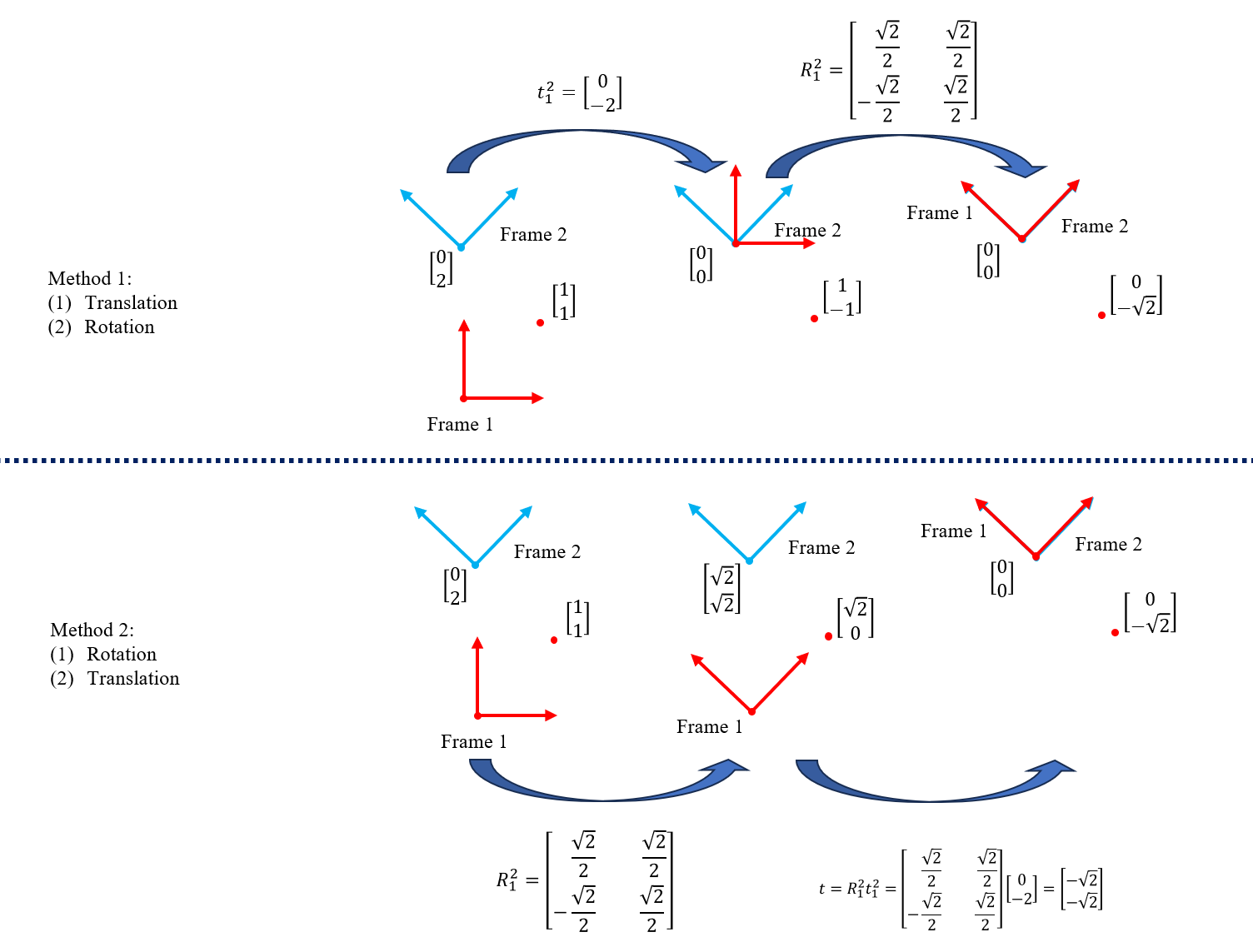
Figure 7.1: A simple example with different origins
We can see that, if we want to use method 1, we can just consecutively do the translation and the rotation. However, if we want to do it reversely, we must multiply the translation by the rotation matrix. Actually it’s easy to show this two methods are equivalent.
In conclusion, the formula is as follows: \[p^2 = R^2_1(p^1+t_1^2) = R^2_1p^1+R^2_1t_1^2\]
7.1.3 Representations of the rotations
Although rotation matrix is enough to characterize a rotation. But it’s not simple enough and not intuitive enough. For example, we can’t explicitly know the rotation angles from the rotation matrix. The rotation matrix has 9 elements, but there are many constraints. So is it possible for us to find a simpler representation for rotation?
7.1.3.1 Euler angles representation
Intuitively, we can achieve any rotation by rotating along the x, y, z axes in turn. First let’s introduce some basic rotations along x,y,z axes.
Proposition 7.3 (Basic Rotations) Below are the basic rotation matrices along the x, y, z axes, all the rotations are counterclockwise.
Rotation along z axes, with angle \(\gamma\) is: \[\begin{bmatrix} &\cos(\gamma) &\sin(\gamma) &0\\ &-\sin(\gamma) &\cos(\gamma) &0\\ &0 &0 &1 \end{bmatrix}\]
Rotation along y axes, with angle \(\beta\) is: \[\begin{bmatrix} &\cos(\beta) &0 &-\sin(\beta)\\ &0 &1 &0\\ &\sin(\beta) &0 &\cos(\beta) \end{bmatrix}\]
Rotation along x axes, with angle \(\alpha\) is: \[\begin{bmatrix} &1&0&0 \\ &0 &\cos(\alpha) &\sin(\alpha)\\ &0 &-\sin(\alpha) &\cos(\alpha) \end{bmatrix}\]
Actually every rotation can be written into combination of no more than three basic rotations, with no two consecutive rotations along the same axis. A popular choice of the sequence is roll-pitch-yaw.
Proposition 7.4 (Roll-pitch-yaw angle representation) Any rotation matrix \(R^w_r\) can be written into combination of basic rotations in the following order:\[R^w_r = R_z(\gamma)R_y(\beta)R_x(\alpha)\] where \(\gamma\) is called the yaw angle, \(\beta\) is called the pitch angle, and \(\alpha\) is called the roll angle.
This representation is very intuitive, because it directly tells us the rotation angles. However, the calculation will include trigonometric functions. So it can be hard to calculate and analyze. Moreover, if you want to recover the Euler angles from rotation matrices, there may be problems in certain point. The example below shows the singularities.
Example 7.4 (Singularities for Euler angles) In formula \[R = R_z(\gamma)R_y(\beta)R_x(\alpha)\] consider \(\beta = \frac{\pi}{2}\). Then we will have: \[R = R_z(\gamma)R_y(\frac{\pi}{2})R_x(\alpha) = \begin{bmatrix} &0 &\sin(\alpha+\gamma) &-\cos(\alpha+\gamma)\\ &0 &\cos(\alpha+\gamma) &\sin(\alpha+\gamma)\\ &1 &0 &0 \end{bmatrix}\] So there are ambiguities in choosing \(\alpha,\gamma\) for the same rotation matrices.
7.1.3.2 Axis-angle representation
Another intuitive representation is the axis-angle representation. Imagine a rotation in 3D space, it seems that all the rotations are rotation with respect to an axis (not necessary to be aligned with the x,y,z axes) for some angle. How to find the axis and the corresponding angle?
Given rotation angle and axis, how can we get the rotation matrix? Next theorem will give us an explicit formula.
Theorem 7.1 (Rodrigues' rotation formula) Given a rotation angle \(\theta\) and a rotation axis \(u\) (expressed by a unit vector). The rotation matrix \(R\) can be computed as: \[R = \cos(\theta)I_3+\sin(\theta)[u]_\times+(1-\cos(\theta))uu^T\] where \([u]_\times = \begin{bmatrix} &0 &-u_z &u_y\\ &u_z &0 &-u_x\\ &-u_y &u_x &0 \end{bmatrix}\)
How can we do it reversely? Intuitively, axis of the rotation is the direction that the rotation preserves. Mathematically speaking, axis of rotation is in the direction of the eigenvector with respect to the eigenvalue of 1. From the discussion above, if rotation is not equal to identity, then there is a unique direction of rotation axis. So we can solve for the rotation axis by calculating \(u\) satisfying:\[Ru = u\] To get the rotation angle, we notice that if we take trace of both of the sides of Rodrigues’ rotation formula, we can get:\[\text{Tr}(R) = 2\cos(\theta) + 1\] Note that if we treat \(\theta\) as the minimal angle of the rotation, we can always restrict the \(\theta\in[0,\pi]\) and thus \(\theta = \arccos(\frac{\text{Tr}(R) - 1}{2})\). However, then we will leave the rotation direction to the sign of axis \(u\). That is to say: \(R(u,\theta)^{-1} = R(-u,\theta)\). So we need to double check the two potential solutions to make sure which rotation is the one we want.
7.1.3.3 Quaternion representation
W.R. Hamilton first introduced the definition of quaternion representation.
Definition 7.2 (Quaternion) A quaternion is represented in the form \(\textbf{q} = \textbf{i}q_1 + \textbf{j}q_2 + \textbf{k}q_3 + q_4\), where \(q_1,q_2,q_3,q_4\) are real numbers and \(\bf i,j,k\) satisfying: \[\begin{align} &\textbf{i}^2=\textbf{j}^2=\textbf{k}^2=-1\\ &\textbf{ij} = -\textbf{ji} = \textbf{k} \quad \textbf{jk} = -\textbf{kj} = \textbf{i} \quad \textbf{ki} = -\textbf{ik} = \textbf{j} \end{align}\]
We can also write the quaternion in the column vector form: \(\textbf{q} = \begin{bmatrix} q_1\\q_2\\q_3\\q_4 \end{bmatrix}\). We are particularly interested in unit quaternions, which means the column vector has unit length. Unit quaternions can represent rotations, actually we can get quaternions immediately from the axis-angle representation. The main idea is to use the axis-angle representation but in a more compact format. Concretely speaking, given rotation angle \(\theta\) and rotation axis \(u\)(in unit length), the corresponding unit quaternion is as follows: \[q = \begin{bmatrix}u\sin(\frac{\theta}{2}) \\ \cos(\frac{\theta}{2})\end{bmatrix}\]
The corresponding rotation matrix is: \[R(q) = \begin{bmatrix} q_1^2 - q_2^2 - q_3^2 + q_4^2 &2(q_1q_2-q_3q_4) &2(q_1q_3 +q_2q_4)\\ 2(q_1q_2+q_3q_4) & -q_1^2+q_2^2-q_3^2+q_4^2 &2(q_2q_3 - q_1q_4)\\ 2(q_1q_3-q_2q_4) &2(q_2q_3+q_1q_4) &-q_1^2-q_2^2+q_3^2+q_4^2 \end{bmatrix}\]
Quaternion representation doesn’t have singularities. But there is still a little ambiguity that \(q\) and \(-q\) always represent the same rotation, which means the quaternion is a double cover of the 3D rotation. Actually, quaternions also give us great convenience in calculation, because of its compact representation. For computational use, we care about: (1)How to compose rotations? (2) How to take inverse for quaternions (3) How to rotate a 3D vector using quaternions?
(1)How to compose rotations?
Consider two quaternions \(q_a = q_{a,1}i +q_{a,2}j +q_{a,3}k +q_{a,4},\ q_b = q_{b,1}i +q_{b,2}j +q_{b,3}k +q_{b,4}\). Then the composition of the corresponding rotation is just the product of two quaternions. Explicitly, \[\begin{align} q_c = q_a\otimes q_b =& (q_{a,4}q_{b,1} -q_{a,3}q_{b,2} + q_{a,2}q_{b,3} + q_{a,1}q_{b,4})i \\ +& (q_{a,3}q_{b,1} +q_{a,4}q_{b,2} - q_{a,1}q_{b,3} + q_{a,2}q_{b,4})j \\ +& (-q_{a,2}q_{b,1} +q_{a,1}q_{b,2} + q_{a,4}q_{b,3} + q_{a,3}q_{b,4})k \\ +& (-q_{a,1}q_{b,1} -q_{a,2}q_{b,2} - q_{a,3}q_{b,3} + q_{a,4}q_{b,4}) \end{align}\]
If we use vector to represent quaternion, we can claim the following formula:
\[ q_c = \begin{bmatrix} q_{a,4} & -q_{a,3} & q_{a,2} & q_{a,1}\\ q_{a,3} & q_{a,4} &-q_{a,1} &q_{a,2} \\ -q_{a,2} & q_{a,1} & q_{a,4} &q_{a,3} \\ -q_{a,1} & -q_{a,2} & -q_{a,3} &q_{a,4}\end{bmatrix} \begin{bmatrix} q_{b,1}\\q_{b,2}\\q_{b,3}\\q_{b,4}\end{bmatrix} \] Similar formula can be derived for \(q_a\).
(2) How to take inverse for quaternions?
Assume that now we have the pose of frame \(r\) with respect to a frame \(w\), i.e. we know \(q_r^w\). How can we get the opposite, i.e. the pose of frame \(w\) with respect to frame \(r\)? The answer is to take the inverse of the rotation. It’s easy to carry out using rotation matrix, but how shall we proceed using quaternions? Let’s remind ourselves that quaternion is nothing but rearranged axis-angle representation. So naturally the inverse is as follows: \[q_w^r = \begin{bmatrix}-u_r^w\sin(\frac{\theta}{2}) \\ \cos(\frac{\theta}{2})\end{bmatrix} = (q_r^w)^{-1}\] This process is also compatible with the quaternion product.
(3) How to rotate a 3D vector using quaternions?
One key question is, given coordinates in one frame, and the pose of that frame in another frame, how can we translate the coordinates? Assume there is a point \(p\), and we know its coordinates in frame \(r\), denoted as \(p^r\). Also we know the pose of frame \(r\) in frame \(w\), denoted as \(q_r^w\). For simplicity, we assume that the two frame share the same origin. How can we get the coordinates of \(p\) with respect to the frame \(w\), i.e. \(p^w\)? We have the following formula: \[p^w = (q^w_r)\otimes\begin{bmatrix} p^r\\1\end{bmatrix}\otimes(q^w_r)^{-1} = \begin{bmatrix} R^w_rp^r\\1\end{bmatrix}\] i.e. we can compute the rotation by first stack an extra entry 1 at the end of \(p^r\), then let \(q^w_r\) act ‘conjugately’ on it.
7.1.4 Miscellaneous topics on rotations
7.1.4.1 Lie group structure of rotations
Actually, on one hand, the set of rotation matrices (\(SO(3)\)) is closed under matrix multiplication (and some other properties), which gives rise to its algebraic structure (which is called ‘group’). On the other hand, the set of rotation matrices has its own topological structure (which is called ‘manifold’). Lie group is both group and smooth manifold, but we’ll not introduce Lie group formally.
Geometrically, thanks to the quaternion representation, we can treat the group \(SO(3)\) as a sphere in 4D, but due to \(R(q) = R(-q)\), we must image there are portals connecting the antipodal points. Locally we can just think it as a sphere. For a sphere, we can imagine that at each point there is a tangent space. The tangent space at the identity is called Lie algebra. Why identity? There is nothing special with identity, just because: (1) Every group has identity. (2) The tangent space at other points can be obtained from identity. Lie algebra is deeply connected with Lie group. Imagine the sphere case, the sphere itself is curved, but we can use coordinates to translate the sphere into a flat map. Lie algebra is a flat space which we can make use of to study about the complicated curved Lie group. We will have some intuition on it by examining \(SO(3)\).
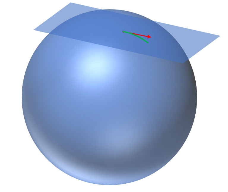
Figure 7.2: Sphere and tangent space
Lie group \(SO(3)\) is related to its Lie algebra \(\mathfrak{so}(3)\). We will state without proof that the Lie algebra \(\mathfrak{so}(3)\) is the set of \(3\times 3\) skew symmetric matrices.
Exponential Map and Logarithm Map:
Looking at the sphere in the picture, it seems natural for us to bridge the endpoint of the green curved line, which is still on the sphere, with the endpoint of the red line, which is in the tangent space. This retraction is called exponential map. For matrix Lie group (including \(SO(3)\)), the exponential map coinsides with the matrix exponential (See A.1.)
We will check this on the \(SO(3)\) case:
Theorem 7.2 (Matrix exponential for rotations) The exponential map \(\text{exp:}\mathfrak{so}(3)\to SO(3)\) is well-defined.
Proof. Consider a \(3\times 3\) skew symmetric matrix \(A = \begin{bmatrix} 0 &-c &b\\c &0 &-a\\-b &a &0 \end{bmatrix}\), define \(w = \begin{bmatrix} a\\b\\c \end{bmatrix}, \hat{w} = w/\|w\|, \theta=\|w\|\). Then \(A = w_\times\). Consider \(\hat{w}_\times\), using the properties of the cross product, we have:\(\hat{w}^3_\times = -\hat{w}_\times\). Thus we can know that: \[\begin{align} \exp(A) &= I + (1-\frac{\theta^3}{3!}+\frac{\theta^5}{5!}+\dots)\hat{w}_\times + (\frac{\theta^2}{2!}-\frac{\theta^4}{4!}+\frac{\theta^6}{6!})\hat{w}_\times^2\\ &= I + \frac{\sin\theta}{\theta}A + \frac{1-\cos\theta}{\theta^2}A^2 \end{align}\] which actually coincide with the Rodrigues’ formula. Thus \(\exp(A)\) is a rotation matrix.
Actually the exponential map for \(SO(3)\) is surjective. From the derivation above, I believe we can see the similarity of this with the axis-angle representation. In order to map backwards, we want to recover the angle and the axis from the rotation matrix. There are infinitely many possible points due to the periodic property of trigonometric functions. So we may restrict the rotation angle \(\theta \in [0,\pi)\)。 Then from the derivation of the axis-angle representation, we can get: \[\begin{align} \theta &= \arccos(\frac{\text{Tr}(R) - 1}{2}) \end{align}\] Next is to recover the axis. Note that the whole space of \(n\times n\) matrices is the direct sum of \(n\times n\) symmetric matrices and \(n\times n\) skew symmetric matrices. So we can decompose the rotation matrix into symmetric and skew symmetric parts. From the formula above, we can decompose as: \[ \exp(A) = \underbrace{\frac{\sin\theta}{\theta}A}_{\text{skew symmetric}} + \underbrace{I + \frac{1-\cos\theta}{\theta^2}A^2}_{\text{symmetric}} \] Thus we can recover the skew symmetric matrix \(A\) (the axis) by taking the skew symmetric part of \(\exp(A)\). Concretely, we can get: \(A = \frac{\theta}{2\sin\theta}(R - R^T)\).
Next we will give an example of how to use exponential map and logarithm map to do interpolation of rotations. Suppose we have two rotations \(R_1,R_2\), and we want to find a rotation \(R\) that is in between. We can use the following formula: \[R = R_1\exp(\lambda\log(R_1^TR_2))\] where \(\lambda\in[0,1]\).
7.2 The Pinhole Camera Model
Next let’s take a look at the pinhole camera model, which is the simplest one. In this model, the picture in 2D is the projection of the corresponding 3D points with respect to the optical center.
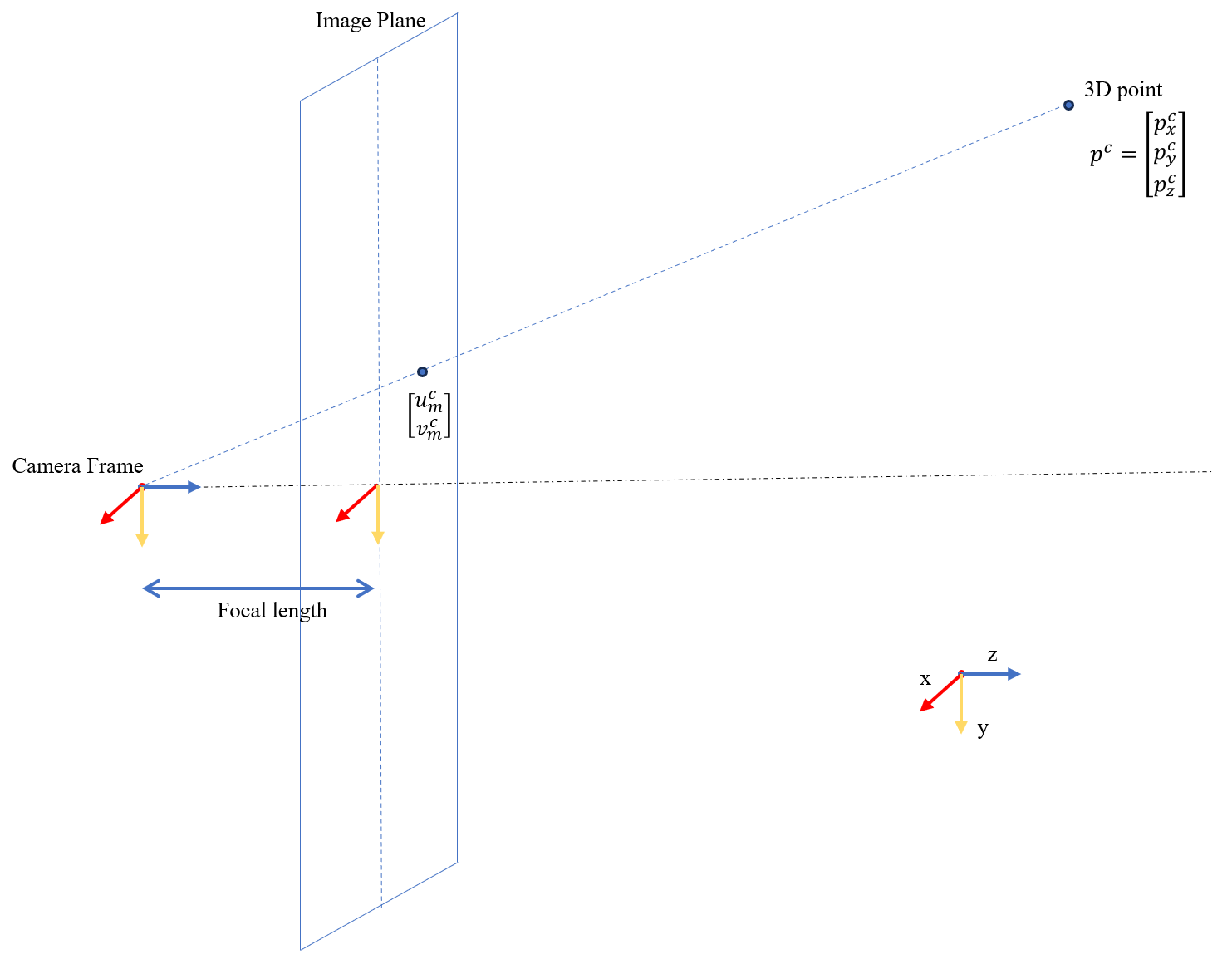
Figure 7.3: Pinhole Camera Model
Consider point \(p\) in the camera frame. Suppose the focal length(i.e. the distance from the optical center to the image plane) is \(f\). Then the coordinates of the projection of \(p\) is: \[p_m^c = \begin{bmatrix} u_m^c\\v_m^c \end{bmatrix} = \begin{bmatrix} f\frac{p^c_x}{p^c_z}\\ f\frac{p^c_y}{p^c_z} \end{bmatrix}\] The unit of these coordinates are meter. We would prefer to write the formula into a matrix form, but the barrier here is the quotient. In order to overcome this, we introduce homogeneous coordinates. In homogeneous coordinates system, if coordinates are multiplied by a non-zero scalar then the resulting coordinates represent the same point. We will add an extra entry to better represent this equivalence. Denote \[\tilde{p^c} = \begin{bmatrix} p_x^c\\p_y^c\\p_z^c\\1 \end{bmatrix}\] Then the equivalence can be expressed as \[\forall k\neq0 \text{,}\quad \ \begin{bmatrix} p_x^c\\p_y^c\\p_z^c\\1 \end{bmatrix} \sim \begin{bmatrix} kp_x^c\\kp_y^c\\kp_z^c\\k \end{bmatrix}\] With this notation, the projection equation can be written as: \[p^c_z\begin{bmatrix} u_m^c\\v_m^c\\1 \end{bmatrix} = \begin{bmatrix} f &0 &0 \\ 0 &f &0\\ 0 &0 &1\end{bmatrix} \begin{bmatrix} 1 &0 &0 &0 \\ 0 &1 &0 &0\\ 0 &0 &1 &0\end{bmatrix} \begin{bmatrix} p_x^c\\p_y^c\\p_z^c\\1 \end{bmatrix}\]
Normally when we deal with points in a 2D picture, we will prefer the unit is in pixels instead of meters. Next we will show how to convert the coordinates into pixels. In convention, the origin of the pixel coordinates is at the top-left of the image. So that we can express the coordinates in pixel as follows: \[\begin{bmatrix} u^I\\v^I\\1 \end{bmatrix} = \begin{bmatrix} s_x &0 &o_x \\ 0 &s_y &o_y\\ 0 &0 &1\end{bmatrix} \begin{bmatrix} u_m^c\\v_m^c\\1 \end{bmatrix}\] where \(s_x\) is the number of horizontal pixels per meter, \(s_y\) is the number of vertical pixels per meter, and \(\begin{bmatrix} o_x\\o_y\end{bmatrix}\) is the coordinates of the optical center.
Combing the previous result, we can get: \[\begin{align} p_z^c\begin{bmatrix} u^I\\v^I\\1 \end{bmatrix} =& \begin{bmatrix} s_x &0 &o_x \\ 0 &s_y &o_y\\ 0 &0 &1\end{bmatrix} \begin{bmatrix} f &0 &0 \\ 0 &f &0\\ 0 &0 &1\end{bmatrix} \begin{bmatrix} 1 &0 &0 &0 \\ 0 &1 &0 &0\\ 0 &0 &1 &0\end{bmatrix} \begin{bmatrix} p_x^c\\p_y^c\\p_z^c\\1 \end{bmatrix} \\ =& \underbrace{\begin{bmatrix} s_xf &0 &o_x \\ 0 &s_yf &o_y\\ 0 &0 &1\end{bmatrix}}_{K} \begin{bmatrix} 1 &0 &0 &0 \\ 0 &1 &0 &0\\ 0 &0 &1 &0\end{bmatrix} \begin{bmatrix} p_x^c\\p_y^c\\p_z^c\\1 \end{bmatrix}\end{align}\] where \(K\) is called intrinsic matrix.
Notice that, in our derivation above, the homogeneous coordinates of \(p\) is in the camera frame. However, it’s not always easy to know the coordinates in the camera frame. For example, sometimes we may have many different camera views, or the camera itself is moving. What we usually have is the coordinate of the 3D points in the world frame. Therefore we will add a procedure to transform the coordinates from world fram to the camera frame. From the previous section, we can know that we just need to do some rotations and translations. Therefore we can obtain the formula: \[\begin{align} p_z^c\begin{bmatrix} u^I\\v^I\\1 \end{bmatrix} =& \begin{bmatrix} s_xf &0 &o_x \\ 0 &s_yf &o_y\\ 0 &0 &1\end{bmatrix} \begin{bmatrix} 1 &0 &0 &0 \\ 0 &1 &0 &0\\ 0 &0 &1 &0\end{bmatrix} \begin{bmatrix} R_w^c &t^c_w \\ 0 &1 \end{bmatrix}\begin{bmatrix} p_x^w\\p_y^w\\p_z^w\\1 \end{bmatrix}\\ =& \begin{bmatrix} s_xf &0 &o_x \\ 0 &s_yf &o_y\\ 0 &0 &1\end{bmatrix} \begin{bmatrix} R_w^c &t^c_w\end{bmatrix}\begin{bmatrix} p_x^w\\p_y^w\\p_z^w\\1 \end{bmatrix} \end{align}\] where the matrix \(\begin{bmatrix} R_w^c &t^c_w\end{bmatrix}\) is called the extrinsic matrix.
Some pinhole cameras will introduce significant distortion to images. For cameras with wide field of view (FOV), they often suffers from radial distortion. Radial distortion makes straight lines look curved in the image. The farther points are from the center of the image, the larger the radial distortion will be. Radial distortion is primarily dominated by low-order components. An easy model of the distortion (in camera frame) is:
\[u^c = (1+K_1r^2+K_2r^4)u^c_{\text{distort}}\quad\quad v^c = (1+K_1r^2+K_2r^4)v^c_{\text{distort}}\] where \((u^c,v^c)\) is the undistorted image point, \((u^c_{\text{distort}},v^c_{\text{distort}})\) is the distorted image point, \(r^2=(u^c_{\text{distort}})^2 +(v^c_{\text{distort}})^2\), and the \(K_n\) is the n-th distortion coefficient.
If we want to express in the image frame, we can obtain the following model: \[u^I = (1+K_1r^2+K_2r^4)(u^I_{\text{distort}}-o_x)+o_x\quad\quad v^I = (1+K_1r^2+K_2r^4)(v^I_{\text{distort}}-o_y)+o_y\] where \(r^2=(u^I_{\text{distort}}-o_x)^2 +(v^I_{\text{distort}}-o_y)^2\).
It’s worth to mention that despite the radial distortion, there is another distortion called tangential distortion, which will not be elaborated here.
We often assume that the intrinsics of the camera and he distortion coefficients are already known from the previous camera calibration process, i.e. we always assume that the camera is calibrated.
There are many existing codes and toolbox by hand if we want to undistort the pictures. Such as OpenCV has undistort function, and Matlab has undistortImage function. They can take in distorted images and return the undistorted ones.
7.3 Camera Pose Estimation
Suppose now we have a calibrated camera, but we don’t know the rotation and translation, i.e. the pose of the camera. We wish to find the extrinsics. Now what we have is a set of \(n\) 3D points and their corresponding 2D image projections. We wish to estimate the pose of the camera from these corresponding points.
7.3.1 The P3P Problem
Let’s start from something simple. Consider there are three points \(P_1^w,P_2^w,P_3^w\) in the world frame, and their corresponding projection points on the image plane \(P^c_{m,1},P^c_{m,2},P^c_{m,3}\). The problem is: Can we found the coordinates of the points \(P_1,P_2,P_3\) in the camera frame? We will introduce a direct way to tackle the problem, called Grunert’s method.
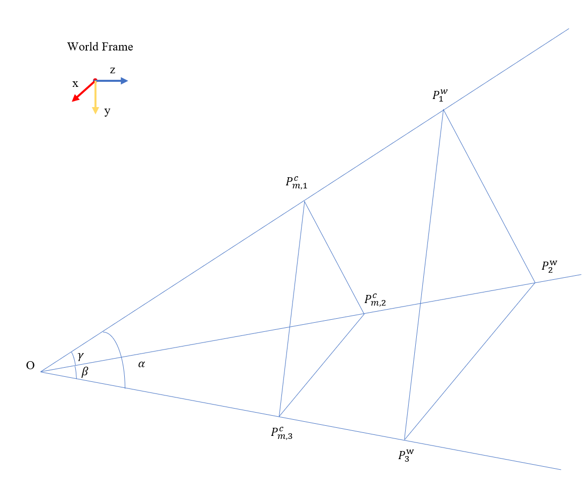
Figure 7.4: P3P problem
From the coordinates of \(P^c_{m,1},P^c_{m,2},P^c_{m,3}\) in the image plane, we can calculate the angles between \(P_1,P_2,P_3\). Denote the angle between \(P_1,P_2\) as \(\gamma\), the angle between \(P_2,P_3\) as \(\beta\), and the angle between \(P_1,P_3\) as \(\alpha\). Remember that if \(P^c_{m,i} = \begin{bmatrix}u_{m,i}^c\\v^c_{m,i}\\1\end{bmatrix}\), then the camera frame coordinates \(P^c_i = \frac{s_i}{\sqrt{1+(u_{m,i}^c)^2+(v_{m,i}^c)^2}}\begin{bmatrix}u_{m,i}^c\\v_{m,i}^c\\1\end{bmatrix}\). So what we have to do is to solve for \(s_i\), which is the distance from the origin to the point \(P_i\).
Using law of cosines, we can obtain:
\[\begin{align} s_1^2 +s_2^2 - 2s_1s_2\cos\gamma = c^2\\ s_1^2 +s_3^2 - 2s_1s_3\cos\beta = b^2\\ s_2^2 +s_3^2 - 2s_2s_3\cos\alpha = a^2\\ \end{align}\]
Then if we let \(s_2 = us_1,s_3 = vs_1\), we can obtain: \[\begin{align} s_1^2 = \frac{c^2}{1+u^2-2u\cos\gamma}\\ s_1^2= \frac{b^2}{1+v^2-2v\cos\beta}\\ s_1^2= \frac{a^2}{v^2+u^2-2uv\cos\alpha}\\ \end{align}\] Then we can get: \[ u^2-\frac{c^2}{b^2} v^2+2 v \frac{c^2}{b^2} \cos \beta-2 u \cos \gamma+\frac{b^2-c^2}{b^2}=0 \] and \[ u^2+\frac{b^2-a^2}{b^2} v^2-2 u v \cos \alpha+\frac{2 a^2}{b^2} v \cos \beta-\frac{a^2}{b^2}=0 \] Then substituting the later equation back to the former one, we can express \(u\) in terms of \(v\). Then plug this into the latter equality, we can finally get an equation: \[ A_4 v^4+A_3 v^3+A_2 v^2+A_1 v+A_0=0 \] where
\[\begin{align} & A_4=\left(\frac{a^2-c^2}{b^2}-1\right)^2-\frac{4 c^2}{b^2} \cos ^2 \alpha \\ & A_3=4\left[\frac{a^2-c^2}{b^2}\left(1-\frac{a^2-c^2}{b^2}\right) \cos \beta-\left(1-\frac{a^2+c^2}{b^2}\right) \cos \alpha \cos \gamma+2 \frac{c^2}{b^2} \cos ^2 \alpha \cos \beta\right] \\ & A_2=2[\left(\frac{a^2-c^2}{b^2}\right)^2-1+2\left(\frac{a^2-c^2}{b^2}\right)^2 \cos ^2 \beta+2\left(\frac{b^2-c^2}{b^2}\right) \cos ^2 \alpha \\ & -4\left(\frac{a^2+c^2}{b^2}\right) \cos \alpha \cos \beta \cos \gamma+2\left(\frac{b^2-a^2}{b^2}\right) \cos ^2 \gamma] \\ & A_1=4\left[-\left(\frac{a^2-c^2}{b^2}\right)\left(1+\frac{a^2-c^2}{b^2}\right) \cos \beta+\frac{2 a^2}{b^2} \cos ^2 \gamma \cos \beta-\left(1-\left(\frac{a^2+c^2}{b^2}\right)\right) \cos \alpha \cos \gamma\right] \\ & A_0=\left(1+\frac{a^2-c^2}{b^2}\right)^2-\frac{4 a^2}{b^2} \cos ^2 \gamma \end{align}\]
From this equation, we can obtain up to four solutions. With each \(v\) we can obtain the corresponding \(u\) and thus all the other parameters. To eliminate the ambiguity, we can use a 4th point to confirm which one is the right solution.